August 17, 2018. I discuss the physics of an inverted pendulum, and prove (using a judicious combination of hand-waving and the Hill determinant) that if you wobble the pivot fast enough, the pendulum will settle into equilbrium upside-down.

Introduction

Prerequisites: basic classical mechanics, Fourier series, differential equations.

Tie a rock to a piece of string, and suspend it from a nail. If you give the rock a little nudge, it will oscillate, with its period going as the square root of the length of the string. Gradually, it will lose energy to air friction and return to its freely hanging, equilibrium position. So the equilibrium is stable. All this is familiar and not particularly interesting.

But here is a much weirder fact about pendulums. If you turn the rock and string arrangement upside down, and wiggle fast enough, the rock will stand on end! Not only that, it will be stable. Someone can nudge it, and it will slowly return to the upright position. Similarly, if I take an ordinary rope, and wobble it fast enough, then not only will it stand on end, but a suitably light fakir could climb up. So classical mechanics can almost explain the famous levitating Indian rope trick. (I say “almost” since “rope” here really means “finite chain of rigid pendulums”. I will discuss this restriction in the next post.)

Single pendulum

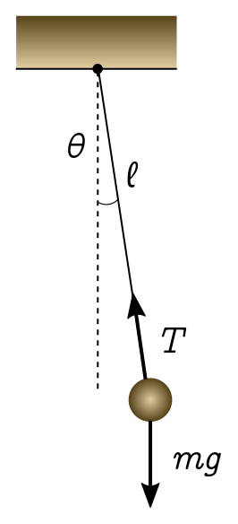
Let’s start by turning a normal pendulum upside down. We have a mass $m$ attached to the end of a rigid, massless rod of length $\ell$, and a pivot which is moving up and down with some time-dependent position $f(t)$. We want to find the equations of motion and figure out if we can wobble the pivot so as to stabilise the pendulum in the upside-down position.

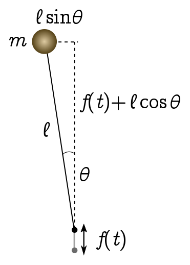
We’ll use Lagrangian mechanics, which is a bit neater than the Newtonian approach here. Recall that the Lagrangian $L = K - V$, where $K$ is the kinetic energy and $V$ the potential energy of the system. There is a single degree of freedom, $\theta$, the displacement of the pendulum from the upright vertical. This translates into $(x ,y)$ coordinates via

\[x = \ell \sin\theta, \quad y = f + \ell \cos\theta.\]

We have a gravitational potential:

\[V = mgy = mg(f + \ell \cos\theta),\]

and kinetic energy

\[K = \frac{1}{2}m v^2 = \frac{1}{2}m (\dot{x}^2 + \dot{y}^2) = \frac{1}{2}m(\dot{f}^2 + \ell^2 \dot{\theta}^2 + 2 \ell\sin\theta \dot{f} \dot{\theta}).\]

The Euler-Lagrange equations yield

\[\begin{align*} \frac{\partial L}{\partial \theta} & = \frac{\partial K}{\partial\theta} - \frac{\partial V}{\partial \theta} \\ & = m \ell g \sin\theta + m\ell \dot{f} \dot{\theta})\cos\theta \\ & = \frac{d}{dt}\frac{\partial L}{\partial \dot{\theta}} \\ & = \frac{d}{dt}\left[m\ell^2 \dot{\theta} + m\ell \sin\theta\dot{f}\right]\\ & = m\ell^2 \ddot{\theta} + m\ell \cos\theta \dot{f}\dot{\theta} - m\ell \ddot{f} \sin\theta. \end{align*}\]

Cleaning up, we find the equation of motion:

\[\ell \ddot{\theta} =g+ \ddot{f}\sin\theta.\]

Note that this is exactly the equation we get for a forced pendulum hanging down, but with $g \to -g$. To make some progress, let’s assume we’re wobbling the pivot up and down with angular frequency $\omega$ and amplitude $A$:

\[f(t) = A \cos(\omega t).\]

Since we are considering perturbations around $\theta = 0$, it makes sense to look at small angles where $\sin\theta \approx \theta$. Then our equation of motion becomes

\[\ell \ddot{\theta} = g- \omega^2 A \cos(\omega t)\theta. \tag{1}\label{eom1}\]

We can make things a bit neater by rescaling time $\tau = \omega t$, and defining new constants $\delta = -g/\omega^2\ell$, $\epsilon = A/\ell$:

\[\frac{d^2\theta}{d\tau^2} + \big[\delta + \epsilon \cos(\tau)\big]\theta = 0. \tag{2}\label{mathieu}\]

This is Mathieu’s equation. It appears all over the place in applied mathematics, from vibrating drumheads and forced pendulums to rocking boats and radio antennae. (See Lawrence Ruby’s article for further discussion of these examples.) This is a tricky equation, with no closed-form solutions built out of elementary functions. In the next section, we will use some clever approximation methods (and a liberal amount of hindsight) to come up with a sharp stability criterion. But before we do that, we can make a guess based on dimensional analysis.

The parameters for the forcing frequency of the pivot are the amplitude $A$ and frequency $\omega$. We expect that making these larger will increase stability. A simple measure of the effect is the product $A\omega$, which has the dimensions of velocity. The two dimensionful constants for the unforced pendulum are $g$ and the length $\ell$, which combine to give $g\ell$, which has dimensions of velocity squared. Making this larger should destabilise the pendulum, since it will want to swing under its own weight. Thus, dimensional analysis suggests the stability criterion

\[g\ell \lesssim A^2\omega^2.\]

We will derive a condition of exactly this sort below.

Parameters and stability

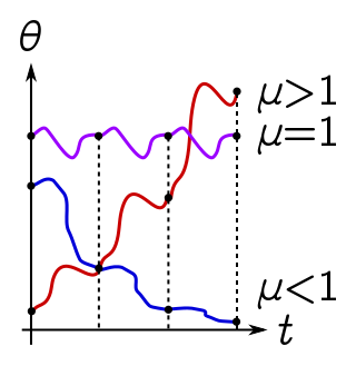
There is a bit of theory needed to rigorously understand the stability of the Mathieu equation. Instead, we will make a sequence of well-motivated guesses which turn out to give the right answer! Here is the basic idea. When we wobble the pivot with a periodic driving function $f(t)$, the pendulum wants to oscillate with the same period, say $T$. But due to a mismatch with the natural frequency of the pendulum, the oscillation may decay by some factor each period:

\[\theta(t + T) = \mu \theta (t), \quad |\mu| < 1.\]

These solutions will be stable, since they decay to the equilibrium configuration we want, $\theta \to 0$. Alternatively, if the natural and forcing frequency line up, we can get resonance, where the oscillations grow exponentially:

\[\theta(t + T) = \mu \theta (t), \quad |\mu| > 1.\]

These resonant solutions are unbounded and hence unstable.

Whether we get unstable or stable solutions depends on the parameters of the problem, in our case, the constants $\epsilon, \delta$ of (\ref{mathieu}). The stable and unstable regions of parameter space will be separated by a boundary corresponding to genuine periodic motion,

\[\theta(t+T) = \theta(t).\]

Our strategy will be to figure out what values of $\epsilon$ and $\delta$ allow for periodic solutions. This will give us the border between stable and unstable regions! (This procedure may strike you as dubious since it hinges on the existence of these solutions which are periodic up to a constant, and I haven’t really justified their existence. As it turns out, their existence is guaranteed by Floquet theory, also known as Bloch’s theorem in a different context. See the references if you want to know more.)

Periodic solutions and the Hill determinant

So, let’s consider an arbitrary solution of period $T = 2\pi$ in the variable $\tau$, which we can expand as a Fourier series:

\[\theta(\tau) = \sum_{n=\infty}^\infty c_n e^{-in\tau}\]

for some unknown, infinite set of coefficients ${c_n}$. Plugging into the Mathieu equation (\ref{mathieu}), we get

\[\begin{align*} 0 & = \frac{d^2\theta}{d\tau^2} + \big[\delta + \epsilon \cos(\tau)\big]\theta \\ & = \sum_{n=\infty}^\infty c_n e^{-in\tau}\left[-n^2 + \delta + \frac{\epsilon}{2}(e^{i\tau}+e^{-i\tau})\right] \\ & = \sum_{n=\infty}^\infty e^{-in\tau}\left[(\delta-n^2)c_n + \frac{\epsilon}{2}(c_{n-1}+c_{n+1})\right], \end{align*}\]

where on the last line, we shift the dummy variable so that $c_n e^{-i(n\pm 1)\tau} \to c_{n\mp 1} e^{-in\tau}$. But we know from the uniqueness of Fourier series that the coefficients of $e^{-in\tau}$ on the LHS and RHS are equal. Thus,

\[c_n + \frac{\epsilon}{2(\delta-n^2)}(c_{n-1}+c_{n+1}) = 0. \tag{3}\label{fourier}\]

For each $n$ we have a linear relation between $c_n$ and $c_{n\pm 1}$. We can therefore think of the equation (\ref{fourier}) as an infinite linear system, with some big matrix $M_{mn}$ acting on the infinite vector of coefficients $c_n$. Let’s define $\alpha_n = \epsilon/2(\delta - n^2)$. Then $M$ equals

\[\begin{align*} M_{mn} & = \begin{cases} \alpha_m & n= m\pm1 \\ 1 & n = m \\ 0 & \text{else} \end{cases}\\ & = \left[ \begin{matrix} \ddots & &&&&& \\ & \alpha_1 & 1 & \alpha_1 & & &\\ & & \alpha_0 &1 &\alpha_0 & &\\ & & & \alpha_1 & 1 & \alpha_1 &\\ & & & & & & \ddots \end{matrix} \right] \end{align*}\]

This linear system only has a nontrivial solution if $\det M = 0$, since otherwise we can invert $M c= 0$ to deduce that $c = 0$. Evaluating this infinite determinant (called a Hill determinant) is somewhat involved. The basic idea is to look at a $(2k+1)\times(2k+1)$ submatrix $M^{(k)}$, centred around $M_{00}$, evaluate the determinant $D_k = \det M^{(k)}$, and take $k$ large (see Exercise 1).

We will use a shortcut. Let’s restrict to the regime of fast, small-amplitude oscillations of the pivot, where $\epsilon, \delta \ll 1$. Then solving for $\det M^{(k)} = 0$ can be written as a relation between $\delta$ and $\epsilon$, with higher $k$ corresponding to higher order corrections in these small parameters. Thus, the leading order behaviour is obtained from $k= 1$! A simple calculation shows that

\[D_1 = \left| \begin{matrix} 1 & \alpha_1 &\\ \alpha_0 &1 &\alpha_0\\ & \alpha_1 & 1 \end{matrix} \right| = -\frac{\epsilon^2}{2\delta(\delta - 1)} + 1.\]

Setting $D_1 = 0$ gives us the boundary between stable and unstable regions, to leading order:

\[\epsilon^2 = 2\delta(\delta - 1) \approx -2\delta,\]

using the fact that $\delta \ll 1$. Thus, the stability boundary for the regime we’re interested in is approximately quadratic $|\delta| \sim \epsilon^2$. (If you’re interested, the higher order corrections are given in Richard Rand’s notes.) We expect that increasing the amplitude of oscillations (increasing $\epsilon$), and increasing the frequency (decreasing $\delta$) will lead to instability, so the region of stability is above the boundary in the $\delta$-$\epsilon$ plane:

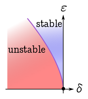
After all this work, we learn that wobbling the pivot of an inverted pendulum at sufficiently high frequency and amplitude will indeed stabilise the pendulum around the inverted position $\theta = 0$. (Note, however, that we require the amplitude to be small compared to the length, $\epsilon = A/\ell \ll 1$, for the perturbative treatment to be valid.) To leading order, stability requires $|\delta| < \epsilon^2/2$. Recalling (\ref{eom1}), this translates into physical requirement that

\[2g\ell < A^2 \omega^2.\]

This only finesses our dimensional analysis by a factor of $2$!

---

Exercise 1. To evaluate the Hill determinant $\det M$, consider a finite $(2k + 1)\times (2k+1)$ submatrix $M^{(k)}$, centred around $M_{00}$:

\[\left[ \begin{matrix} 1&\alpha_k &&& \\ \alpha_{k-1}&1&\alpha_{k-1}&& \\ &\ddots&\ddots&\ddots& \\ &&\alpha_{k-1}&1&\alpha_{k-1} \\ &&&\alpha_k &1 \end{matrix} \right].\]

Let $D_k = \det M^{(k)}$, and use induction to show that the $D_k$ obey the recurrence relation

\[D_{k+3} = (1-\alpha_{k+2}\alpha_{k+3})D_{k+2} + \alpha_{k+2}\alpha_{k+3}(1-\alpha_{k+2}\alpha_{k+3})D_{k+1} + \gamma_{n+1}^2\gamma_{k+2}^3\gamma_{k+3}D_k.\]

The Hill determinant is obtained, in principle, by solving the recurrence and taking $k \to \infty$. In practice, we solve the recurrence numerically, choosing $k$ large enough to get the accuracy needed for our application.

---

Two other points are worth mentioning. First, there are additional regions of stability and instability in $(\delta,\epsilon)$ space which come from setting the Hill determinant to $0$.

Second, we can use the Hill determinant to solve a generalisation of (\ref{mathieu}) called Hill’s equation,

\[\ddot{\theta} + f(t; \vec{\beta}) \theta = 0,\]

where $f$ is any periodic function in time $t$, with some vector of parameters $\vec{\beta}$. We again get regions of stable and unstable “psuedoperiodic” solutions (by Floquet theory), separated by periodic solutions. We plug a Fourier series into the equation, write out the resulting equations as an infinite linear system, and demand that the Hill determinant vanish. This will gives us the stability boundaries in the $\vec{\beta}$ parameter space.

Next time

In the next post, I’ll look at a beautiful theorem of David Acheson which uses different methods to show that a chain of rigid pendulums, oscillated at suitable amplitude and frequency, can be stabilised in the upside-down position. I’ll also talk about the experimental realisations of this phenomenon. They reveal something that our perturbative analysis cannot tell us: how far the pendulum can fall and still return to the inverted equilibrium position. It turns out to be surprisingly large!

References

• “Inverted Pendulums”, §VI.4 Princeton Companion to Applied Mathematics (2015), David Acheson.
• Non-equilibrium statistical mechanics (2016), Andrew Melatos and Andy Martin.
• “Mathieu’s equation” (2016), Richard Rand.
• “Applications of Mathieu equaton” (1995), Lawrence Ruby.