Introduction

Suppose there are $n$ bets I can make, with the return per dollar for bet $k$ represented by a random variable $B_k$ with expected value $\mu_k = \mathbb{E}[B_k]$. If I invest $\omega_k$ on bet $k$, and have a fixed total $\Omega$, then I can view the value of my portfolio as a random variable

If I try to optimize the expected return $\mu_P = \mathbb{E}[P]$, I get a boring linear function

To maximize this, introduce a Lagrange multiplier $\gamma$ to enforce the fixed total:

This is linear and has no local maxima, so the maximal return must lie at the edge of the feasible region. In fact, it’s clear that we just invest all our money in the bet with maximum return:

But putting all your eggs in one basket seems like a bad idea. My intuition is that to optimize my portfolio, my investment should include a spread of high-risk, high-return and low-risk, low-return bets. What have we missed?

Derisky business

Maximizing expected return ignores the risk altogether! The simplest way to measure the risk of our portfolio is the total variance,

If the bets are independent random variables, then the variance is additive, with

where $\sigma^2_k$ is the variance of $B_k$. If they are not independent, then we add covariance terms:

Instead of just maximizing expected return, we should balance return and risk. A simple way to do this is to maximize the convex combination of $\mu_k$ and $-\sigma^2_P$, which we’ll call the $\lambda$-derisked return:

The expected return is $0$-derisked, while $1$-derisked return minimizes the variance of the portfolio and ignores the return completely.

Distributing eggs

For simplicity, let’s assume our bets are independent. Otherwise, we simply diagonalize the covariance matrix and go to a basis of orthogonal bets. Then adding a Lagrange multiplier as above, we get

The partial derivatives are

so we have an extremum at

To determine the value of $\gamma$, note from our constraint that

Since $\gamma \simeq \lambda$, for small $\lambda$ (a return-oriented investor) we can ignore that $\gamma$ term. Then the investments

so we weight investments proportional to expected return, but inversely to variance. Sounds sensible! On the other hand, when $\lambda \to 1$ (a risk-averse investor), the Lagrange multiplier $\gamma \gg (1 - \lambda)\mu_k$, so that the investment is proportional to the inverse variance only:

Intermediate values of $\lambda$ interpolate between these two regimes, with a degeneracy at $\lambda = 0$ where only expected return matters. Thus, we have a whole one-parameter family of risk-sensitive ways to value a portfolio!

Introduction

Say I want to estimate a perfect power like $67^{13}$, but don’t have a calculator. If this isn’t sufficient motivation, it’s easy to make the power so large that no calculator will give you an answer! How do I go about approximating it? I’ll build up a few techniques that are sufficient for an order of magnitude estimate, and even a significant digit or two.

Perfect powers

The first step is to relate single-digit powers to powers of $10$. For instance, as commonly known to coders, $2^{10} = 1024 \approx 10^3$, so we can approximate binary powers easily enough. Here’s a list of tricks for $2$ to $7$, omitting powers of $2$ and $3$:

Also, for good measure:

We can use these to give quick and dirty estimates. For instance,

If you get a calculator out, you find the answer is in fact

so this is correct to the nearest order of magnitude. Great! But clearly, by replacing $6.7$ by $7$ on the second line we are going to overestimate. Can we do better? The rest of this post is devoted to exploring techniques for doing this, but if you’re happy with order of magnitude, stop here.

Binomial boost

The binomial theorem gives us a way to improve these estimates. In general, we have

So, for instance,

using the estimate from the previous section. This is much better! We’ve ignored the factor of $70/2^6$, which means we’ve underestimated, but we’ve also replaced $7^{12}$ with $(100/2)^6$, which is an overestimate, and the two almost cancel. As an exercise, you can use the binomial approximation to check this.

In doing a binomial expansion, where should you stop? Depends on how much precision you want. Here, I went to third order since it gave terms of size $\sim 0.01$, which is the precision I wanted to try and match the correct answer above. How did I know? Well, I know terms in the expansion have the form

so for $n = 13$ and $x = -0.3/7$, progressive terms shrink by $\sim 0.04$ give or take. So I can probably stop after a term of the size I want, in this case, the third term, which was order $\sim 0.01$.

Fast factors

There are other ways to skin this cat. Another strategy is factoring to a simpler number nearby. In our case, we can note that

Then

using our trick $6^9 \approx 10^7$ on the third line. Again, we can improve this estimate by binomially expanding from $66^{13}$ to $67^{13}$, a task I leave for the diligent reader. Taking just the leading term in this second binomial expansion gives $5.3 \times 10^{23}$, a decent improvement. I’m not sure I like this method better — it involves two expansions — but it does illustrate the utility of factoring.

Lucky logs

The last method we’ll look at is logarithms. Here, we use the fact that

so if we know $\log_{10}n$ we immediately have an order of magnitude estimate. We can use log laws

where $\ln$ is the natural logarithm, and the Taylor expansion

Let’s use these to estimate $\log_{10} 67$. We’ll also exploit the fact that $\ln 10 \approx 2.3$. From log laws, we have

We now focus on the Taylor expansion. Since $0.67 \approx 1 - 1/3$, we can write

So we get an index

So we recover our order of magnitude estimate

Evaluating the mantissa with a calculator, we get

so this method is comparable in accuracy to our binomial expansions. In both cases, we kept terms up to $x^3$, so this is about what we expect.

Magic mantissas

The disadvantage of the log method is that it’s a bit hard to see what the mantissa is. Hard, but not impossible! One method is to use the Taylor series for the exponential:

This turns out to be a bit messy to use directly, because the index is large and you need to include a bunch of terms in the expansion to get stable digits. Instead, we we split $0.725 = 0.7 + 0.025$, and deal with $0.7$ first:

since $5^3 = 125$. The cute thing is that we have just used facts from our “power table”. We can use the exponential expansion for the remaining $0.025 = 1/40$, with

using only the leading term in the expansion. We then multiply to find

as claimed above!

Introduction

The Greek philosopher Protagoras famously stated that “man is the measure of all things”. He was also skeptical about whether math could be applied to the real world. According to Aristotle, he arged that “perceptible lines are not the kind of things the geometer talks about”. We’ll make a bad Protagoran joke and use humans, the “measure of all things”, to measure distances by exploiting the geometry of “perceptible lines”.

Theory

So, consider a distant object you want to find the distance to. Hold your hand out at a fixed distance from your eyes and fixed orientation (e.g. horizontal), and estimate the size of the object in fingers $f$. (For best results, use an integer number of fingers.) Your arm and hands form a triangle which is similar to the triangle formed by the distant object:

If $a$ is the length of your arm, $h$ the actual height, $d$ the distance to the object and $f$ the apparent height in fingers, then

Now walk $s$ steps towards the object, so that it has finger width $f’$. We now have a new set of similar triangles:

The ratio of sides now obeys

where we measure distance in steps. We can rearrange $(\ref{f})$ and $(\ref{fdash})$ to eliminate the length of the arm, $a$, and physical height $h$, to find a method for distance measurement about which Protagoras might have mixed feelings.

Practice

Take the transition from $f = 3$ to $f’ = 4$. In this case, the distance estimate is

or four times the number of steps. I find this works with $90$-$95\%$ accuracy for distances on the order of $50$ steps. I suspect that varying finger width and step length are the main source of error; arm length $a$ can be fixed by maximally extending the arm, and orientation of the hands can be fixed by a reference line, e.g. the horizon.

Beyond varying width, the main disadvantage of fingers as a measurement device is their resolution. By counting the number of steps from $f = 9$ to $f’ = 10$, you estimate $d \approx 10s$, but that is the best you can do. For large ratios, you need to replace fingers with a finer measurement instrument, such as a clear plastic ruler held at arm’s length. Although you will get better results and enable yourself to measure larger distances, you may look a tad eccentric. But as Protagoras informs us, that is a tradeoff that each individual must assess themselves.

Extension

It’s simple to extend this method to estimate height. Once $d$ is known, we can use $(\ref{f})$ to give the physical height (or width, or whatever we’ve measured) in terms of other quantities:

Now, if we know $a$ in finger lengths, we will get an estimate of the height in steps. That’s a bit silly, so I suggest learning your arm length, finger width, and step size in meters. But note that, for an order of magnitude guess, one step is around $1.2$ arm lengths, so the height is $1.2$ times the number of steps times the finger span.

Example: I estimated a car had size $f = 3 \text{ fingers} \approx 4 \text{ cm}$ at a distance $d = 40$ steps. This leads to a height estimate

which is probably an overestimate but in the right ballpark. Once again, a ruler leads to more accurate results at the cost of visible dorkiness.

Some general phenomena are named after specific instances. For instance, a mondegreen is a misallocation of word boundaries, with “Lady Mondegreen” a misallocated variant of “laid him on the green”. Another example is the Baader-Meinhof effect, where something is encountered, apparently for the first time, then suddenly noticed everywhere. In 1994, a man called Terry Mullen wrote to a newspaper to describe his experience of frequency bias with the eponymous Marxist guerilla group. In a beautifully self-referential moment, this caused people to begin noticing the Baader-Meinhof effect everywhere! For our purposes, the most important example is the eggcorn: a semantically motivated mishearing, named for “eggcorn”, a cute but infelicitous rendition of “acorn”.

We can lump these under the general heading of “instance-naming” (distinct from synechdoches or metonyms where whole may stand for part as well as vice-versa). A few months ago, I set myself the challenge of self-reflexively naming the phenomenon after an instance, and became promptly stuck. How could I name it after an instance without getting confused with the original referent? And if I came up with a new term, how could it refer to an instance? It seemed impossible. If you like, you can have a go before you read on to my proposed solution.

I forgot about this puzzle until a plane flight last week, where lack of other amusements forced me to solve it. The idea is simple: punningly allude to an instance so as to indicate both the general phenomenon of instance-naming, and a specific example. After some experimentation, I struck on the idea of modifying “eggcorn” to “egcoin”, which literally means “a new word based on an example”. As a semantic equation:

It gets better: on hearing “egcoin”, someone might mistakenly suppose they had heard “eggcorn”. This makes “egcoin” an eggcorn precisely when it is heard as such!

Overview

Consider an integral transform with kernel $K(x, y)$. In general, this gives two distinct transforms,

where $T_i$ integrates over argument $i$, and $\Omega_i$ denotes the corresponding domain of integration. If everything is smooth enough to swap integrals (i.e. Fubini’s theorem), then

For a symmetric kernel $K(x, y) = K(y, x)$ and $\Omega_1 = \Omega_2 = \Omega$, we have $T_1 = T_2 = T$, and our result simplifies to:

From a pure math standpoint, we’ve basically just observed that the integral transforms $T_1$ and $T_2$ are dual,

with respect to a suitably defined inner product $\langle \cdot, \cdot\rangle$. But this turns out to be a useful trick for doing real-life integrals!

Full disclosure. I didn’t come up with this hack, but stole it (with some customizations) from Ramanujan. Also, I’m ignoring many mathematical subtleties! The joys of being a physicist.

The Voigt integral

Let’s take everyone’s favourite example, the 1D Fourier transform:

We can consult a table and pick out, for instance, the pairs

Then our kernel trick gives

The RHS is straightforward to express in terms of the complementary error function:

We complete the square, defining $2\alpha u = x + 2\alpha^2\beta$ to find

We can finally conclude that

I call this the “Voigt integral”after the related convolution in spectroscopy.

Mordell integrals

Here’s a fancier example, again using the Fourier transform. Consider the Mordell integral

with $\Im(\tau) > 0$ to ensure convergence. Note that this is a product of functions which are self-dual under the Fourier transform, up to a change in their parameters:

The kernel trick (and the change of variable $x = 2\pi u$) now gives

This seems like a neat result!

Introduction

It’s a running joke among mathematicians that there are no boring numbers. Here’s the proof. Let $B$ be the set of boring numbers, and suppose for a contradiction it is non-empty. Define $b = \min B$ as the smallest boring number. Since this is a highly unusual property, $b$ is interesting after all! Joke it may be, but there is a sting in the tail. By thinking about how the joke works, we will be led to some rather deep (and perhaps disturbing) insights into set theory and what it can and cannot tell us about the mathematical world.

Integers and rationals are interesting

The joke implicitly uses the fact that “numbers” refers to “whole numbers”

If it didn’t, then the minimum we used to get our contradiction wouldn’t always work! For instance, say we work with the integers

The set of boring integers $B_\mathbb{Z}$ may be unbounded below. Does this cause a problem? Not really. We can just define the smallest boring number as the smallest element minimising the absolute value, i.e.

(The $\text{argmin}$ might actually give us two numbers, $\pm b$, so the negative one is the smallest.) Thus, there are no boring integers. What about boring rational numbers? This is somewhat more elaborate, but if $B_\mathbb{Q}$ is the set of boring rationals, we can define the “smallest” boring number as

where $a/b$ is a fraction in lowest terms. Once again, there may be multiple minimisers of $|a| + |b|$, but only a finite number, so we can choose the smallest. We conclude there are no boring rationals. This pattern suggests there are no boring real numbers. We should be able to find some function with a finite number of minima, and then choose the smallest, right? I’m going to argue that no such function can ever be described. Then I’m going to explain why it might exist anyway, depending on which axioms of set theory we use!

Most real numbers are boring

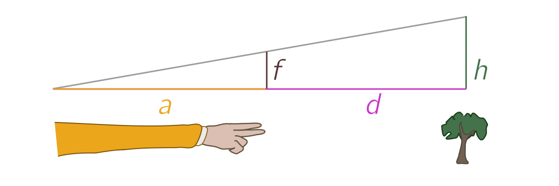
“Boring” and “interesting” are subjective. We’ll use something a tad more well-defined, and replace “interesting” with describable. A number is describable if it has some finite description, using words, mathematical symbols, even a computer program, which uniquely singles out that number. For instance, $\sqrt{2}$ is the positive solution of $x^2 = 2$, $\pi$ is the ratio of a circle’s circumference to its diameter, and $e$ is the limit

It turns out that almost every real number is indescribable, or “boring”, in our official translation of that term. The argument is very simple, and proceeds by simply counting the number of finite descriptions. Each such description consists of a finite sequence of symbols (letters, mathematical squiggles, algorithmic instructions), each of which could be elements of some very large alphabet of symbols. For instance, the text

can be converted into (decimal) unicode as

8730 50 32 105 115 32 116 104 101 32 112 111 115 105 116 105 118 101
32 115 111 108 117 116 105 111 110 32 111 102 32 120 94 50 61 50 46

Imagine some “super unicode” which lets us converts any symbol into a number. The super unicode alphabet may be arbitrarily large, so we will take it to consist of every natural number $\mathbb{N}$. Then a finite description using any symbols can be written as a sequence of the corresponding natural numbers, a trick I will call “unicoding”. To find the number of finite descriptions, we just count the sequences! There is a nice scheme for showing that these are in one-to-one correspondence with the natural numbers themselves, and hence countably infinite. We take a sequence, say

and convert the first bracket and all commas into $1$s, and each number into the corresponding number of $0$s:

In turn, this can be converted to decimal, $66144$. Going in the other direction, any whole number can be written in binary and then converted into sequence:

becomes $(0,1,0,2,0,1,1,1,0,5,2)$. Thus, we have a simple, explicit correspondence between finite sequences of natural numbers and the natural numbers themselves. This basically completes the proof, for the simple reason that there are infinitely more real numbers than there are natural numbers. This is established by Cantor’s beautiful diagonal argument, which I won’t repeat here. The upshot is that, via unicoding and then the binary correspondence, finite descriptions can only capture an infinitesimally small fragment of the real numbers. Most literally cannot be talked about.

The set $B_\mathbb{R}$ includes almost every real number, though quite definitely not every real number you can think of. But, armed with our previous jokes, it’s tempting to think that we can waltz in and make the same joke about $\mathbb{R}$, simply plucking out the smallest element of $B_\mathbb{R}$. Of course, that won’t quite work, because the set need not be bounded below. So instead, suppose there is some explicit function $f$ such that $b \in B_\mathbb{R}$ is the smallest minimizer of $f$, i.e.

If I knew $f$ explicitly, we’d have a description of $b$ after all. Contradiction! But the contradiction here does not imply $B_\mathbb{R}$ is non-empty. After all, most of $\mathbb{R}$ is indescribable for simple set-theoretic reasons. Instead, it means that there cannot be any explicit function $f$. More generally, there cannot be any explicit rule which, given a subset of $\mathbb{R}$, gives some unique number. If there was, we could apply it to $B_\mathbb{R}$ and get the same contradiction. (See Appendix A for discussion of the related Berry paradox.)

An existential aside

There’s a loophole here. Our argument doesn’t establish that $f$ doesn’t exist, just that it has no finite description. And although it might seem weird to trust in the existence of something that we can’t really talk about, we do just this with the real numbers! I believe in all the real numbers, even the ones I can never describe. Is this reasonable? It depends who you ask. There is a philosophy of mathematics called intuitionism which tells us that mathematics is a human invention, and therefore enjoins us to only reason about the things we can construct ourselves. No indescribable real numbers if you please!

I’m not sure about this “mathematical creationism”, and think there are more things in the mathematical heavens than are dreamt of in our finite human philosophy. Why should human limitations be mathematical ones? That said, it’s not the case that anything goes. We should have some firm basis for believing in the existence of those things we can’t discuss, and for the real numbers, the firm basis is drawing a continuous line on a piece of paper, or thinking about infinite decimal expansions. These are models of the real numbers, concrete-ish objects which capture the essence of the abstract entity $\mathbb{R}$. They convince us (or at least me) that there is nothing magical stopping someone from drawing certain points on the line, or continuing certain expansions forever.

Similarly, the indescribable things we would like to exist and reason about in set theory might depend on our models of set theory! I won’t get into the specifics, but an important point is there are many different models of set theory, with different properties, and it seeks unlikely that any one model is right. These properties are abstracted into axioms, formal rules about what exists and what you can or can’t do with sets. Because models of set theory are deep, highly technical constructions, most of the time we go the other way round, and play around with axioms instead. Only later do we go away and find models which support certain sorts of behaviour. The point of all this is to make it a bit less counterintuitive when I say that the existence and properties of boring numbers depend on which axioms we decide to use.

All real numbers are relatively interesting

So, let’s return to our problem of boring real numbers. We argued there was no explicit, finitely describable rule for picking an element out of $B_\mathbb{R}$. But we can always make the existence of such a rule — describable or not — an axiom of our theory! There are two ways to go about doing this. Note that in the first example of boring natural numbers, we use the minimum of the set. We had to be a bit more clever with the integers and rationals, but it essentially boiled down to creating a special sort of ordering on the set, so that any subset (including the boring numbers) has a smallest element. We wrote this is in a complicated way as

for some function $f$, but we could just as well write

where $\mathcal{W}$ denote this ordering on the big set. To be clear, for the integers it is

and for the rationals it is

This is called a well-ordering. Although it may not be describable, we could simply require, as an axiom of set theory, that any set can be well-ordered! More explicitly,

Any set $A$ has a well-ordering $\mathcal{W}_A$ such that any subset of $A$ has a unique minimum element with respect to $\mathcal{W}_A$.

Although it doesn’t spoil our conclusion that most real numbers are boring, such an axiom would allow us to turn the old joke into an argument that all real numbers are relatively interesting, where “relatively interesting” means that there is a finite description where we are allowed to use the well-ordering $\mathcal{W}$. The proof goes as you might expect: let $B^{\mathcal{W}}_\mathbb{R}$ be the set of relatively boring numbers, i.e. numbers with no finite explicit description, even when allowed to use the well-ordering $\mathcal{W}$. Since $\mathcal{W}$ is a well-ordering, we can define

End of proof! So, although most real numbers are strictly boring, with a well-ordering all of them are relatively interesting.

Choosing an order

Well-ordering is not usually treated as an axiom. Historically, set theorists prefer to use a simpler rule called the axiom of choice, which is logically equivalent, as we will argue informally in a moment, but somehow less suspect. As Jerry Bona joked,

The axiom of choice is obviously true and the well-ordering principle obviously false.

(Actually, Bona’s joke mentions a third equivalent form called Zorn’s lemma, but it would confuse matters too much to explain.) Loosely, the axiom of choice just says we can pick an element from a non-empty set. Pretty reasonable huh? If a set is nonempty, it has an element, so we can pluck one out. In fact, it’s usually stated in terms of a family of sets $A_i$, where the subscript $i$ ranges over some indexing set $I$:

Given a family of nonempty sets $A_i$, $i \in I$, we can collect a representative from each set, labelled $f_i \in A_i$.

The well-ordering principle implies the axiom of choice, since I can just take the union of all the sets $A_i$, well-order it with $\mathcal{W}$, and then define $f_i = \min_{\mathcal{W}} A_i$. That’s my set of representatives! The other way round is conceptually straightforward. To well-order a set $A = A_0$, start by choosing an element $f_0 \in A_0$ by the axiom of choice. Then remove it to define a new set $A_1 = A_0 - \{f_0\}$, and select another element $f_1 \in A_1$. Continue in this way, at each stage simply deleting the element from the previous stage and choosing a new one, using

as long as the set is nonempty. The well-ordering is simply the elements in the order we made the choice:

There are two issues with this construction. The first is that it might feel sketchy to use the axiom of choice “as we go” to build the sets, rather than starting with a pre-defined family. But no one said this wasn’t allowed! Second, our method only seems to work for sets as most as large as the natural numbers, since we indexed elements with $n \in \mathbb{N}$. But we can extend it to an arbitrary set using a generalisation of natural numbers called ordinals. We loosely sketch how this is done in Appendix B. Once the dust settles, we find that the axiom of choice is equivalent to well-ordering.

Conclusion

The overarching theme of this post is how much mileage we can get from a bad joke. The answer: quite a lot! We learned not only that there are no boring integers and rational numbers, but via a simple counting argument, that the vast majority of real numbers are indescribably boring. This is equivalent to having no explicit way to well-order the reals. On the other hand, by giving ourselves the ability (via the axiom of choice) to pluck elements at will from non-empty sets, we are able to supply the reals with a well-ordering. So, all reals are relatively interesting, even if we can’t talk about them.

Acknowledgments

As usual, thanks to J.A. for the discussion which led to this post, and also for proposing an elegant mapping analogous to unicoding.

Appendix A: the Berry paradox

Consider the phrase

The smallest real number with no finite, explicit description.

If “smallest” refers to an explicitly definable well-ordering of the reals, then this would seem to pick out a unique number with a finite, explicit description. Contradiction! We used this to argue no explicit well-ordering exists. But let’s compare this to the Berry paradox, which asks us to consider the phrase

The smallest positive integer not definable in under sixty letters.

This phrase clocks in at under sixty letters, and would seem to define a number. Contradiction! Since “smallest” here makes perfect sense (we are dealing with positive integers), to resolve the Berry paradox, we must assume either (a) there is no set $B$ of numbers not definable in under sixty letters, analogous to the original boring number joke, or (b) Berry’s phrase somehow fails to define a number. The most popular solution seems to be (b), on the grounds that referring to the set makes it some kind of “meta-definition”, rather than a definition per se.

Of course, this seems be committed to a very specific notion of “definition”, but the problem persists if we replace “definable” with “meta-definable”, since the smallest non-meta-definable number is really a meta-meta-definition. Let $B^{(0)}$ be the set of numbers not definable in under sixty letters, $B^{(1)}$ the numbers not meta-definable in under $70$ letters, and in general, $B^{(n)}$ the numbers not meta${}^{(n)}$-definable in under $60+10n$ letters. We call any number in the union of all these sets $\mathcal{B} = \cup_{n\geq0} B^{(n)}$ “lim-definable”. This is closed under the operation of going meta. Now consider the phrase

The smallest positive integer not finitely lim-definable.

Since lim-definability is closed under going meta, as is “finite”, this is now a definition at the same level. Option (b) is no longer available to us, so only option (a) remains, and it follows that, like the joke that began it all, all positive integers are finitely lim-definable. This is of course obviously true.

Our argument against an explicit well-ordering is very closely related to the Berry paradox. The point of considering lim-definability is that we can build the same descriptive hierarchy for the real numbers, take the union, and rule out option (b). This leaves two ways to avoid a contradiction: no lim-definable ordering exists (involving some finite but unbounded number of references to sets in the hierarchy), or like the Berry paradox, every real is lim-definable. But unlike the positive integers, we know from set theory that the second option can’t be true! We still have a countable number of lim-definitions, as we can argue from unicoding. So there must be no lim-definable ordering of the reals, and no explicit well-ordering in particular.

Appendix B: ordinals and the axiom of choice

Ordinals are sets which we use to stand in for numbers. The smallest ordinal is $0$, which is defined as the empty set $\varnothing = \{\}$. Each ordinal $\alpha$ has a unique successor $\alpha + 1$, defined by simply appending a copy of $\alpha$ to itself:

To illustrate, we apply the successor operation to $0 = \varnothing$ a few times:

Going on in this way gives us all the finite ordinals, but there are also infinite ordinals. The smallest infinite ordinal, conventionally denoted $\omega$, can be identified with the natural numbers:

It is called a limit ordinal since it is not the successor of any finite ordinal. It is bigger than all the finite ones, $n < \omega$. The successor is defined as before,

thereby giving a precise meaning to “infinity plus one”! We won’t say more about the structure of these ordinals. The main point is that we can always “count” the elements in a set $A$ using ordinals, no matter how big it is. Let’s now return to the problem of proving the axiom of choice implies that any set $A$ can be well-ordered. The basic idea is to start with $0$, but keep on counting up “past infinity”, defining

for any ordinal $\alpha$. The resulting set of representatives, labelled by ordinals, is

with $f_\alpha < f_\beta$ just in case the ordinals $\alpha < \beta$. This is a well-ordering since the cardinals are themselves well-ordered. Now, we’ve skipped many important technical details, but the main point was that the argument looks pretty similar to the previous one!

Introduction

In calculus, the regular derivative is defined as the local gradient of a function:

We will abbreviate this as $f’ = Df$, understanding that $f$ is a function of $x$ and $D$ differentiates with respect to $x$. We can always differentiate again, and again, and in fact as many times as we want. Using our new notation, we can write the $n$th derivative as

This is well-defined as long as $n$ is a whole number. But what if we could consider other types of derivatives, say half a derivative? Let’s call this $D^{1/2} = \sqrt{D}$. In the same way that applying two ordinary derivatives gives the second derivative, it seems reasonable to hope that two half derivatives give a full derivative:

What could half a derivative look like?

To be continued

The easiest way to go about this to use a trick called analytic continuation. This has a precise meaning in complex analysis, and we’re going to do something similar in spirit, but not quite as rigorous. The basic idea is to find some nice, specific function we can differentiate $n$ times, and which happens to give us a nice answer in terms of $n$. We then define the fractional derivative $D^\alpha$ acting on this function by replacing $n$ with $\alpha$. A sanity check will be that, for general $\alpha, \beta$, the fractional derivatives obey

so, e.g., two half-derivatives give a full derivative, $\sqrt{D}\cdot \sqrt{D} = D$. We call this property multiplicativity after the identical-looking rule for indices. There are two issues with this approach. First, how do we extend the definition to general functions? And second, are the definitions for different functions in agreement? In general, the answers are very complicated, but in this post, I’ll consider the two simplest methods for defining fractional derivatives. This means we can talk about the functions they apply to, and check they agree, without a huge technical overhead.

Our first nice function is the exponential $e^{\omega x}$. Differentiating simply pulls down a factor of $\omega$ each time, so

It’s very clear, then, how to define the fractional derivative acting on this:

Great! We can easily check the multiplicative property, assuming that constants pass through the derivatives:

Now, you might think this is useless because we can only take fractional derivatives of exponential functions. But at this point, we introduce another assumption, namely that the fractional derivatives are linear:

where $f_1, f_2$ are functions and $\lambda_1, \lambda_2$ are constants. In particular, let’s suppose this linearity applies to an infinite collection of exponentials multiplied by constants $\lambda$, arranged into an integral

Then by linearity,

Functions which can be written this way are said to have a Fourier representation, with the function $ \lambda (\omega)$ the Fourier transform. Most functions have one! Let’s do a very simple example: the sine function, bane of high school trigonometry classes everywhere. What is its half derivative? We start by writing sine in terms of exponentials as

We then take a half-derivative using our exponential rule and linearity:

There are a few things to note. First, this is not a real function, so in general, half derivatives of a real functions need not be real. It should also be clear there is some ambiguity about which roots we choose. In general this ambiguity is harmless, and we just take the principal values (with arguments between $-\pi$ and $\pi$), but this issue will crop up any below in a subtle way. Finally, observe that we can just as easily do crazy things like take $i$ derivatives! We set $\alpha = i$, so the $i$th derivative of sine is

since the principal values are

I’m not sure if this has any applications, but it’s cute. I invite the interested reader to take $\pi$ derivatives of sine. What better way to celebrate $\pi$ day!

Fractorials

Exponentials aren’t the only nice functions we can use to define fractional derivatives. In fact, a more common approach is to use powers. The first function we encounter in high school is usually the identity function, $f(x) = x$. From there, we build up to polynomials $x^m$, and then arbitrary powers $x^s$. The derivative of a power has a very simple form:

If we differentiate again, we bring down a factor of $s - 1$ and reduce the index again. And so on and so forth. This leads to the expression for $n$ derivatives:

So far, this doesn’t look like something we can easily continue to non-integer values of $n$. But let’s assume for a moment $s$ is an integer. Then we can write

where we have used the good old factorial function $s!$. Thus, we can write

To analytically continue this, we need a beautiful object called the Gamma function $\Gamma$. We’ll define it properly below, but for the moment, the only properties we need are that (a) it agrees with the factorial function at (shifted) integer values,

and (b) is defined for non-integer values as well. I like to think of it as the “fractorial” because it makes sense for fractional arguments! In addition to delightfully bad puns, the Gamma function lets us write

and immediately continue to the fractional derivative:

Too easy! Once again, we can check the multiplicative property:

So this gives us another, evidently different way to define fractional derivatives. It will apply to any sum or integral of powers of $x$, for instance, infinite polynomials called power series, and their close cousins the Laurent series which include reciprocal powers:

These cover a lot of ground, and there is an even more general object called the Mellin transform, analogous to the Fourier transform. But we won’t go there. Instead, let’s do another simple example. One of the interesting properties of the Gamma function is that it blows up to (minus) infinity for nonpositive integers:

This is actually essential to get sensible answers! For instance, let’s take the derivative of a constant, $1 = x^0$. Then according to our definition,

since the $\Gamma(0)$ in the denominator makes the whole thing vanish. More intriguingly, these infinities sometimes cancel in sensible ways. For instance, if we take a derivative of $1/x$, we should get $-1/x^2$. If we plug $x^{-1}$ into our formula, it gives

Both the numerator and the denominator blow up, which should make us queasy. But there is a trick here. It turns out that for any $z$, the Gamma function obeys the functional equation

Since $\Gamma(k + 1) = k!$, this gives the usual relation for factorials,

It also gives the sneaky result $\Gamma(0) = (-1)\Gamma(-1)$. Both $\Gamma(0)$ and $\Gamma(-1)$ blow up of course, but in the derivative of $1/x$, the $\Gamma(-1)$ terms cancel, leaving $(-1)x^{-2} = -1/x^2$ as required.

Gamma and tongs

This all sounds great, but you might be wondering why the Gamma function is the right way to extend the factorial function away from whole numbers. In fact, any old function that interpolates between them would also work and satisfy the multiplicative property. What we’re going to do in this last section is use the fractional derivatives, defined using exponentials, to derive the Gamma function continuation. And in order to this, we have to grit our teeth and define the Gamma function in all its glory:

If you’re interested, you can find proofs of the functional equation and so on elsewhere. Instead, we’re going to make the sneaky change of variables $t = \omega x$, yielding

If we change $s \to -s$, and rearrange, we get a formula for $x^s$ in terms of exponentials:

Great! Now we just go ahead and use rule (\ref{exp}), with the hope we will get rule (\ref{power}). As usual, we proceed using linearity:

where on the last line we used (\ref{gamma}), but with $s -\alpha$ instead of $s$. This isn’t quite what we want. To make progress, we’ll take advantage of the reflection formula for the Gamma function (derived here for instance):

We can apply this to both $\Gamma(-s)$ and $\Gamma[-(s-\alpha)]$ to get

This is almost (\ref{power}), the thing we were after! But there is this strange factor with sines out the front. Recall the definition of sine in terms of complex exponentials. This lets us write the funny factor as

It would be magical if that $(-1)^\alpha$ could somehow behave differently and cancel the $\alpha$ terms floating around, right? Well, turns out it does! We can write $-1 = e^{\pm \pi i}$, and hence

I won’t spell out the details, but if you look at this proof of the reflection formula, the two different terms in the sine arise from parts of an integration contour which lie in almost the same place, but where we take roots in different ways. In particular, evaluating $(-1)^\alpha$ gives $e^{\pm \pi i \alpha}$ respectively, so they cancel the $\alpha$ terms after all. The upshot is that our funny factor is just unity:

Thus, our exponential rule actually reproduces the rule for powers of $x$ involving the Gamma function! Now, to be clear, fractional derivatives are a big and mathematically heavy topic, and I’ve only skimmed the surface. But it’s neat that the two simplest approaches agree.

Acknowledgments

Thanks to J.A. for chatting about fractional derivatives, and getting me thinking about the simplest way to define them.

Introduction

Fermi approximation is the art of making good order-of-magnitude estimates. I’ve written about them at greater length here and here, but I’ve never really found a satisfactory explanation for why they work. Order-of-magnitude is certainly a charitable margin of error, but time and time again, I find they are better than they have any right to be! Clearly, there must be an underlying statistical explanation for this apparently unreasonable effectiveness.

Products and log-normality

There are two key techniques: the use of geometric means, and the factorisation into subestimates. We start with geometric means. Suppose a random variable $F$ is a product of many independent random variables,

Then the logarithm of $F$ is a sum of many random variables $Y_i = \log X_i$:

By the central limit theorem for unlike variables (see e.g. this post), for large $N$ this approaches a normal distribution:

where the $Y_i$ have mean $\mu_i$ and variance $\sigma_i^2$. We say that $F$ has a log-normal distribution, since its log is normal.

Geometric means

In Fermi estimates, one of the basic techniques is to take geometric means of estimates, typically an overestimate and an underestimate. For instance, to Fermi estimate the population of Chile, I could consider a number like one million which seems much too low, and a number like one hundred million which seems much too high, and take their geometric mean:

Since population is a product of many different factors, it is reasonable to expect it to approximate a log-normal distribution. Then, after logs, the geometric mean $\sqrt{ab}$ becomes the arithmetic mean of $\log a$ and $\log b$:

Taking the mean $\mu$ of the distribution as the true value, these geometric means provide an unbiased estimator of the mean. Moreover, the error of the estimate will decrease as $1/k$ for $k$ samples (assuming human estimates sample from the distribution), so more is better. To see how much better I could do on the Chile population estimate, I solicited guesses from four friends, and obtained $20, 20, 30$ and $35$ million. Combining with my estimate, I get a geometric mean

The actual population is around $18$ million, so the estimate made from more guesses is indeed better! This is also better than the arithemetic average, $23$ million. Incidentally, this also illustrates the wisdom of the crowd, also called “diversity of prediction”. The individual errors from a broad spread of guesses tend to cancel each other out, leading to a better-behaved average, though in this case in logarithmic space.

In general, Fermi estimates work best for numbers which are large random products (this is how we try to solve them!), so the problem domain tends to enforce the statistical properties we want. For many examples of log-normal distributions in the real world, see Limpert, Stahel and Abbt (2001). It’s worth noting that not everything we can Fermi estimate is log-normal, however. Many things in the real world obey power laws, for instance, and although you can exploit this to make better Fermi estimates (as lukeprog does in his tutorial), we can happily Fermi estimate power-law distributed numbers without this advanced technology.

Are Fermi estimates unreasonably effective in this context? Maybe. But the estimates work best in the high-density core where things look uniform, not out at the tails, and it’s not until we get to the tails that the difference between the log-normal and power law (or exponential, or Weibull, or your favourite skewed distribution) becomes pronounced. So the unreasonable effectiveness here can probably be explained by the resemblance to the log-normal, though this is something I’d like to check more carefully in future.

The philosophy of subestimates

Now we’ve dealt with geometric means and log-normality, we turn to the effectiveness of factorising a Fermi estimate. If we take logarithms, factors become summands, and we’ll reason about those since they are simpler. If $Z = X + Y$ is a sum of independent random variables, the variance is additive, so that

Thus, splitting a sum into estimates of the summands and adding them should not change the variance of the guess. Of course, there is a fallacy in this reasoning: humans are not sampling from the underlying distribution! When we guess, we introduce our own random errors. For instance, my estimate for $Z$ will have some human noise $\varepsilon_Z$:

Similarly, my guesses for $X$ and $Y$ have some random errors $\varepsilon_X$ and $\varepsilon_Y$. There is no reason for the variances of $\varepsilon_X$ and $\varepsilon_Y$ to add up to the variance of $\varepsilon_Z$. The sum could be bigger, or it could be smaller. But a good decomposition should reduce the combined variance:

If log-normality is the science of Fermi estimates, picking variance-reducing subestimates is the art. But I suspect that $\hat{Z}$ roughly speaking behaves like a test statistic for $Z$, with the number of samples corresponding to how many data points for $Z$ we have encountered. So we expect that $\text{var}(\varepsilon_Z)$ will vanish roughly as $1/k$ with $k$ samples. If we have more exposure to the distributions for $X$ and $Y$, the combined error will probably be smaller. This is why we carve into subfactors we understand!

Variance reduction in practice

I’ll end with a speculative rule of thumb for when to factor: try generating over- and underestimates for the factors and the product, which in additive notation give

where $\Delta$ refers to the difference of the (logarithm of the) over- and underestimate. Factorise if the first estimated error is smaller than the second. Let’s illustrate by returning to the population of Chile. I can try factoring it into a number of regions multiplied by the average number of people per region. Taking logs (in base $10$) of the over- and underestimate of Chile’s population I gave above, I get

On the other hand, for regions I would make a lower guess of $5$ and an upper guess of $30$, with a difference in logs of $(\Delta X)^2 = 0.6$. For regional population, I would make a lower guess of $5\times 10^5$ and an upper guess of $5\times 10^6$, with $(\Delta Y)^2 = 1$. Thus,

The guess from the factorisation (taking geometric means) is

This is even better than the crowdsourced estimate! For reference, the number of regions is $16$, while our estimated mean is around $12$, and the average population per region is a bit over a million, which we’ve mildly overestimated at $1.6$ million. The two balance out and give a better overall estimate.

Conclusion

From a statistical perspective, Fermi estimates are based on two techniques: geometric means and splitting into subfactors. We usually estimate things which can be expressed as a product of many factors. These will tend towards a log-normal distribution by the (log of the) central limit theorem, so that geometric means provide a good estimator, exactly like the usual mean for normally distributed variables. Subestimates, on the other hand, carve guesses into factors we understand, i.e. have more data points for, so that (assuming they behave like test statistics) variance is reduced. The effectiveness of Fermi estimates is quite reasonable after all!

Introduction

Explanations must come to an end somewhere.

Reductionism is the idea that you explain stuff with smaller stuff, and keep going until you stop. In many ways, this describes the explanatory program of 20th century physics, which, starting from the 19th century puzzles of statistical mechanics, conjured up atoms, subatomic particles, the zoo of the Standard Model, and even tinier hypothetical entities like strings and spin foams. Most physicists spend their time in a lab, on a computer, or in front of a blackboard, trying to reduce complex things to simple things they understand. So like Platonism in mathematics, reductionism in physics simply makes a philosophy out of everyday practice. We break stuff down, so things reduce; we play abstractly with mathematical objects, so they exist abstractly.

But also like Platonism, reductionism is a convenient fiction, or rather, a caricature in which some things are emphasised at the cost of others. And given the reverence which which philosophers hold the considered ontological verdicts of science, it’s worth asking: what does science really tell us about the universe? What sorts of objects are necessary for explanation? Does explanation go only upwards, or can it go downwards or sideways? Should we eliminate the things we explained? And what has explanation to do with existence anyway? This post is an attempt to unconfuse myself about some of these questions.

The existence of shoes

… our common sense conception of psychological phenomena constitutes a radically false theory, a theory so fundamentally defective that both the principles and ontology of that theory will eventually be displaced, rather than smoothly reduced, by completed neuroscience.

Physical objects can be described at different levels. A shoe is constructed from flat sheets of material, curved, cut, marked, and stuck together in clever ways; materials curve and stick by virtue of their constituent chemicals, usually long, jointed molecular chains called polymers; polymers, in turn, are built like lego from a smorgasboard of elements; and each elemental atom is a dense nuclear core, surrounded by electrons whirring around in elaborate orbitals.

From the properties of the neutrons, protons and electrons, it seems we can work our way upwards, and infer everything else. The laws of quantum mechanics and electromagnetism determine the orbital structure of the atom. The valence shell of the atom determines how it can combine with other atoms to form chemicals. Finally, the structural motifs and functional groups of the polymers gives it the properties the industrial chemist, the designer, and the cobbler exploit to make a shoe. Thus, some philosophers conclude, only electrons, protons, and neutrons exist. The rest can be eliminated as unnecessary ontological baggage. This view is called eliminative reductionism. It is a hardcore philosophy which does not believe in shoes [¹].

There is a gentler, less silly form of reductionism which grants the existence of shoes, but insists that they are (in the phrase of Jack Smart) nothing “over and above” the constituent subatomic particles. The shoe “just is” electrons and protons and neutrons, in some order; this is what we mean by a shoe. There are others way to characterise the reduction, and a whole literature devoted to the attendant subtleties, but most fall under the heading of analytic micro-quibbles. Instead, we will make a much simpler observation: order matters.

Clearly, if we took those subatomic particles, and arranged them in a different way, we would get different elements, different chemicals, and a duck or a planetesimal instead of a shoe. Arrangement is important. It is patently absurd to try and explain the bulk properties of the shoe—the fact that it fits around a human foot, for instance—without appeal to arrangement, since a different order yields objects which do not fit around a foot. Since order has explanatory significance, it should presumably be tarred with the same ontic brush we apply to things like electrons.

Of course, one may object that explanation does not equal existence. I can handily account for the continual disappearance of my socks by the hypothesis of sock imps. But this is a bad explanation! It’s not consistent with other reliably known facts about the world. Sock imps don’t make the ontic cut, not because there is no link between explanation and what we deem to exist, but because that link should only be made for robust explanations, and the poor little sock imps collapse at the first empirical hurdle. That different arrangements of things have different properties is robust, almost to the point of truism, and there seems to be no principled reason to ban order from our ontology.

Emergence vs structure

More is different.

It’s worth noting the parallel to emergence. In his famous article “More is Different”, Philip W. Anderson argued for the idea of domain-specific laws and dynamical principles which did not follow the strict, one-way explanatory hierarchy of reduction, particularly in his field of condensed matter physics. And indeed, condensed matter makes a science of order itself, studying how properties of macroscopic wholes (such as phases of matter) “emerge” from the arrangement of microscopic parts. Anderson thought of emergence as patterns that appear when you “zoom out” from the constituents, but which are still made from the constituents; we are just describing those constituents at a different level.

But this seems to suffer from the same problem as a reductionist account of shoes. The “emergent properties” are not properties of the constituents at all! The symmetries, order parameters, and collective excitations studied by condensed matter physicists belong only to the arrangements. In fact, systems made from totally different materials can exhibit the same emergent behaviour [²]! They are something new, something “over and above” the spins of the lattice, or the carbon atoms of a hexagonal monolayer, since different arrangements of those same parts would have different properties. We can turn Anderson’s snappy slogan around: different is more. If arranging things differently gives them new and different properties, it is a sign of structure, and structure is something over and above the component parts themselves.

What is a particle?

It is raining instructions out there; it’s raining programs; it’s raining tree-growing, fluff-spreading, algorithms. That is not a metaphor, it is the plain truth. It couldn’t be any plainer if it were raining floppy discs.

We don’t need emergence to argue for structure; we can use the elementary components themselves. When philosophers talk about reductionism, they tend to imagine subatomic particles as small, indivisible blobs, without internal organisation or further ontological bells and whistles. An electron might have properties like mass or charge, and obey the curious dictates of quantum mechanics, but all this is packaged irreducibly and not worth further discussion. But if we try and unpack all these “simple” properties, we will find that, like the magic bag of Mary Poppins, a particle is much deeper than it first appears! The Large Hadron Collider does not produce evidence for tiny, structureless blobs. Rather, it confirms at a rate of petabytes per second that the universe is made of mathematics.

The state-of-the-art definition of a particle is a bit of a mouthful: an irreducible representation of the Lorentz group. In plain English, being a representation means that particles are objects which have or “transform with” symmetries, in the same way a circle looks the same however you rotate it. That it is irreducible means that it cannot be split into smaller parts which have the same symmetry, which is the mathematical avatar of being “indivisible”. Finally, the symmetry itself, the Lorentz group, is the same group describing the shape of empty space according to special relativity. So, in summary, a particle transforms with the symmetries of empty space, and cannot be split into parts with this symmetry. Lurking implicitly in the background is the whole framework of quantum mechanics, and in particular, that particles are states in a Hilbert space. In plain English, we can add and subtract states of a particle, and compare them to each other.

Thus, every particle is like a mathematical diamond: indivisible, multifacted, and structured up to the hilt. When philosophers of science eagerly assent to believe whatever the particle physicists tell them, they may not realise what they signed up for! Spacetime, quantum mechanics, and symmetries, the Lorentz group and Hilbert spaces; these are all welded indissolubly to form the most robust and fundamental objects in the universe. Even with something as “simple” as an electron, order is inescapable.

Unreasonable effectiveness and natural patterns

It is difficult to avoid the impression that a miracle confronts us here, quite comparable… to the two miracles of the existence of laws of nature and of the human mind’s capacity to divine them.

It may feel like we have jumped from physical to mathematical objects in one fell, tendentious swoop. Do we need Hilbert space, or might another mathematical concept suffice? And does Hilbert space really exist, or is it merely a useful human invention? If the latter, why so useful? This is intentionally designed to rhyme with our earlier statement that order is a robustly explanatory feature of the world, and distinct from the things that are ordered. Mathematics really just is the study of order, or patterns, according to their own peculiar and abstract logic. Physics (and to a lesser extent the other sciences) study natural patterns, the way these structures or forms of order are realised in the natural world. That applies not just to emergent behaviour like phases of matter, but even the crystalline makeup of an elementary particle.

I have tried to motivate this perspective from the nature of physical explanation, but perhaps it can teach us about mathematical explanation and its relation to the physical world. A common criticism of Platonism is that, if mathematical objects exist in some non-physical realm, the ability to do mathematics must involve extrasensory perception. Clearly, since we are physical beings, this ability is grounded in physical experience, and now we have a simple explanation: patterns are naturally realised everywhere, from cardinal numbers in counting cows to topology in tying a knot to representation theory in colliding protons. We don’t need magical access to the World of Forms to see these things; they are all around us.

Similarly, the unreasonable effectiveness of mathematics for describing the world, first noted by Eugene Wigner, seems no more miraculous that the utility of integers for counting loaves of bread rather than proving results about number theory. We get the patterns from the world, clean them up, rebrand a little, and start connecting them together. The meta-patterns that emerge are remarkable, but the appearance of “unreasonable effectiveness” is the result of a largely successful PR campaign to divorce mathematical structures from their physical origins. As Einstein quipped, “Since the mathematicians have invaded the theory of relativity, I do not understand it myself anymore.” The abstraction of pseudo-Riemannian geometry follows from the more concrete act of bouncing light off mirrors.

More and more, we are seeing this converse of unreasonable effectiveness, where deep mathematical ideas are inspired by physics. The living embodiment of this trend is Ed Witten, a string theorist whose contributions to mathematics have been so profound and wide-ranging that he earned a Fields Medal (the Nobel prize in mathematics), the only physicist to have ever done so! Once again, there is no mystery here; it is just the usual state of affairs, but without the Platonist guff to distract us. The patterns are out there and always have been.

What is a pattern?

Everything comes to be from both subject and form.

All this raises the question: what is a pattern? The first and most famous philosophical treatment of these issues is the hylomorphism of Aristotle, who argued that objects are a compound of both form (the structure, order, or patterns I have discussed here) and matter (energy or “raw potentia”). I won’t discuss Aristotle’s ideas in greater detail. Suffice to say they have deeply informed this post, and the interested reader should check out James Franklin’s modern take. Instead, I will approach the question by picking on two smaller problems, taking Newton’s laws as a concrete example.

Newton formulated his laws of motion (such as $F = ma$) in terms of forces and acceleration. Does the empirical robustness of these laws mean that this is the only way to formulate them? Not at all! There are two other distinct but equivalent versions of classical mechanics: Lagrangian and Hamiltonian. They explain the same things, make the same predictions, and thus seem to describe the same natural patterns. This suggests to me that although patterns are discovered, formalisms are invented. A pattern is the equivalence class of descriptions.

Students of physics will be aware that, although Hamiltonian and Lagrangian mechanics are equivalent to Newton’s laws in the mechanical context, they have taken on a life of their own. The Lagrangian approach involves the mathematics of optimising functions, while the Hamiltonian approach in its most abstract form becomes the mathematical field of symplectic geometry. Both Lagrangian and Hamiltonian mechanics can be upgraded (with some inspired retrospective guesswork) to frameworks for quantum mechanics, which Newton’s laws simpliciter cannot. There is much more going on than a simple isomorphism of description! A more nuanced view is that humans invent formalisms which can agree on a domain of interest, a restricted equivalence class of explanation if you will. But the formalisms will tend to grow beyond the selvage lines of the original use case. Formalisms are only perspectives on patterns.

This hints at certain structural “metalaws”. Patterns are big and rhizomatic; human-invented mathematical frameworks are a single mathematical glance, if you like, and can only take in part of the pattern. Even if formalisms agree on some domain, they will suggest different corridors of growth. A rectangle may be both an equiangular quadrilateral, or a parallelogram with diagonals of equal length, but the notions involved and corresponding generalisations are distinct. This also helps explain the phenomenon of deep connections between apparently unrelated mathematical objects, sometimes only revealed by a clever change of perspective. It could be that there is a paucity of structure, so that by dumb luck (and the pigeonhole principle), we often unknowingly describe the same thing in a different guise. But to my mind, it is more likely that patterns tend to sprawl and overlap in complex ways. They are less like a few items of furniture in a crumbling garret—paucity of structure—and more like the interwined flora of a tropical jungle.

The second issue is how accurate our descriptions must be. We know that Newton’s laws are not exactly correct, and break down in regimes far-removed from those of everyday experience, such as the very small (where quantum mechanics applies) or the very fast (where special relativity applies). Does this mean we should stop believing in forces, or Lagrangians, or Hamiltonians? This is like the old Platonist quibble that there is no such thing as a perfect circle in the real world, so we must be reasoning about circles in some other realm. In both cases, the pattern is only approximately realised in nature, with bumps and fuzzy edges. But approximation is itself subject to structural laws, exhibiting patterns treated by mathematics (in, e.g., topology) and physics (effective field theory). Perhaps an even better example is statistics, which is literally all about extracting structure from noisy realisations. So structural approximations are clearly robust, lawlike and explanatory, even if they are subtle. Incidentally, this suggests another metalaw: patterns can stand in patterned relations to other patterns.

This ties back to our original question about the nature of physical explanation. Reductionism instructs us to boil things down to their smallest elements. The Aristotelian view is that, really, we should be searching for form and structure at whatever level they happen to occur. This is not only the nature of emergence, but physics more broadly. How else can we connect the study of the large-scale structure of spacetime, quarks, bowling balls, planetesimals, or storm clouds? Physicists almost never boil things down to their smallest elements! Rather, it seems much more accurate to say that they look for patterns “in the wild”. (In contrast, mathematicians study patterns “in captivity”, which gives them that air of artifice and pedigree.)

One upshot is that, for better or worse, physicists often wade into other disciplines armed with the lassoo of an Emergent Pattern to corral the apparent complexity. See for instance scaling laws, self-organised criticality, small-world networks, and thermodynamic explanations for life itself. They’re not always right (and they’re not always respectful), but they are just doing their thang.

Conclusion

I’ve argued that the nature of physical explanation is richer and less boringly hierarchical than the reductionist would have us believe. In order to explain the properties of shoes or particles, it seems not only parsimonious but necessary to commit to the existence of patterns in addition to the things which make those patterns up. This not only jives with (and ontologically grounds) the notion of emergence, but also provides a handle on the metaphysics and epistemology of mathematical explanation. Put simply, mathematicians study patterns; physicists study natural patterns.

Clearly, I’ve left many questions unanswered. Must patterns be instantiated in the physical world, and if not, where do such patterns live? What is the “mereology” that allows them to combine, or to recursively describe their relationships? And finally, what grounds the truth about patterns, in physics, mathematics, or elsewhere? Most of these I defer to Aristotle, though I hope to write more in future. In the mean time, discussion and debate are welcome!

Acknowledgments and references

I’d like to thank Leon Di Stefano for introducing me to Aristotelian structuralism and many enriching conversations over the years. His ideas inspired and informed this post. I’ve also been heavily influenced by James Franklin’s book, An Aristotelian realist view of mathematics. Aristotle himself writes with characteristic brevity on form and matter in Physics (i). Finally, I fitfully consulted the SEP entries on reductionism and mathematical structuralism.

Introduction

The binomial approximation is the result that, for any real $\alpha$, and $|x| \ll 1$,

The usual proof involves calculus. Here, we present a sketchy shortcut and an elementary longcut, neither of which involves calculus, strictly speaking. We also derive the quadratic term, and end with a fun party trick for finding roots.

Sketchy shortcut

We begin with the shortcut. In an earlier post, I derived the following result for the exponential, and $|x| \ll 1$:

Rather than go off and read the post, we can do even better and simply define the exponential by this property. If it’s true, then for any $r$, we can set $x = r/n$ for very large $n$ to get

In the limit of infinite $n$, the expression should be exact. And indeed, this is the standard definition of $e^r$:

Let’s proceed with a proof of the binomial approximation. The natural logarithm is the inverse function, so that

Recall that

Thus, taking the logarithm $(1 + x)^\alpha$, we have

and hence

This works since all the corrections are at higher order in $x$.

Elementary longcut

This is a bit high brow, and we can get to the same conclusion using simple algebra. First note that, from the binomial theorem,

for $|x| \ll 1$, neglecting higher order terms which are much smaller. So the binomial approximation is true for whole numbers $n$. If we consider a fraction $q = m/n$, then $(1 + x)^q$ raised to the power $n$ should equal

by the binomial theorem. Let’s assume

with some higher order terms we can ignore. Raising to the power $n$, we can use the binomial approximation for $n$ to get

Comparing to (\ref{m}), we find that $\beta = m/n$, and hence the binomial approximation is true for positive rationals. We can add negative powers using the geometric series:

and hence for a negative rational $q = -m/n$,

as required. Finally, there is arbitrary real $\alpha$. This is actually trivial, in some sense. Unlike whole numbers (repeated multiplication), fractions (roots), or negative numbers (reciprocals), an irrational power has no obvious interpretation. The most reasonable thing to do is define it as a limit of rational powers that approximate it:

where $q_n$ is a sequence of rational numbers (e.g. the decimal expansion) approximating $r$. In this case, the binomial approximation gives

and so the result holds for all real numbers.

Higher terms

It’s possible, if messy, to extend these methods to determine the next term in the approximation. We’ll do the longcut, and use big-O notation, with $O(x^3)$ in this context meaning “terms with powers of $x^3$ or higher”. The binomial theorem gives

since the coefficient of the $x^2$ term is the number of ways of choosing $2$ items (the $x$ terms) from $n$ items (the factors in the power). For a rational $q = m/n$, we have

and if we assume

then the binomial theorem again gives

The coefficient of the linear term $nq = m$ matches, but the quadratic term requires more work. Comparing to (\ref{second}) and rearranging for $\gamma$, we have

Thus, we find that to second order,

The extension to real and negative powers is easy. The extension to higher terms in $x$ is not. They obey something called the binomial series,

and I have no idea how to get this without calculus. (One can use “analytic continuation” but this feels too much like cheating to me, partly because it’s not clear why this continuation is unique.) Any tips appreciated!

Rooting out the answer

The applications are many and various, but the simplest thing we can try is quickly calculating powers $y^\alpha$. The general trick is to find a power near $y$ that is simpler to evaluate, factor out the simple answer, then use the binomial approximation. I think there are actually better ways to estimate positive powers, but the binomial approximation really shines in the estimation of roots. It can even be a good party trick, depending on the kind of parties you go to!

Suppose someone asks you to find the square root of $8$. You look for a nearby perfect square, in this case $9$, then factor eight into $9$ times one minus something small:

We can take $\alpha = 1/2$ and $x = -1/9$ in the binomial approximation, and see how we go, noting that

To first order, we get

To second order,

The actual answer is $\sqrt{8} = 2.828$, so even the first term in the binomial approximation is very good! We’ll finish with a somewhat more involved example. Let’s approximate the fifth root of six, $6^{1/5}$. I only know one fifth power of the top of my head, $2^5 = 32$, and this happens to be near $6^2 = 36$. We can chain these observations together as follows:

At this point, we could separately approximate $\sqrt{2}$, but I happen to know it’s about $1.414$, so I can divide by $90$ (or even just $100$ for a quick mental estimate), and add them together to get

Consulting a calculator, this is correct to two decimal places! With the power of the binomial approximation, you can do it in your head.