October 16, 2020. Night thoughts on Kepler’s first law. Main takeaway: an elliptical orbit is just simple harmonic motion with respect to inverse radius! I review Kepler’s laws and derive the second and third for good measure as well.

Kepler’s laws

I’ve always found Kepler’s laws a mixed bag. Here they are in their full glory:

1. The orbit of a planet is an ellipse with the sun at one focus.
2. Planets sweep out equal areas in equal time.
3. The square of the orbital period is proportional to the cube of the semi-major axis.

Everything is fairly simple if we replace the ellipse with a circle. The focus is the centre, where the sun (which I’ll take to be much heavier than the planet) sits, and the semi-major axis is just the radius $r$. Kepler’s second law is simply the statement that the planet orbits at a fixed speed $v$, and the relation between orbital period and orbital radius implies

\[T^2 = \left(\frac{2\pi r}{v}\right)^2 \propto \frac{r^2}{v^2} = \frac{r}{a},\]

since centripetal acceleration is $a = v^2/r$. In order for this to be proportional to $r^3$, we need $a \propto r^{-2}$, which is how Newton arrived at his inverse square law:

\[a = \frac{F}{m} = \frac{GM}{r^2}.\]

So far so good. The messiness comes from the fact that the first law allows for more mysterious elliptical orbits! Where the heck do these come from? Last night, I was finding it hard to sleep when a sweet hack occurred to me. Read on to find out what it was!

Angular momentum

As opposed to Newton, who started with Kepler’s laws, we are going to go in the other direction, and use Newtonian physics to get the ellipses. First, let’s recall the basics of angular momentum. Suppose an object of mass $m$ is at a distance $r$ from some point, and has an angular velocity $\omega = d\theta/dt$. Then the angular momentum $L$ is

\[L = mr^2 \omega = m \cdot \frac{r^2\, d\theta}{dt}.\]

If $L$ is fixed, then in a fixed, small time increment $dt$, $r^2\, d\theta$ is fixed. But this is twice the area swept out! We simply calculate the area of the corresponding circle at that radius:

\[dA = \pi r^2 \cdot \frac{d\theta}{2\pi} = \frac{1}{2} r^2 \,d\theta.\]

While $r$ itself can change a little, this contributes a negligible amount as $dt$ gets small. Adding all these changes up, we find Kepler’s second law: equal areas are swept out in equal times. Once again, Newton used this to learn about conservation of angular momentum. We will, instead, assume conservation of angular momentum, which indeed holds for a central force like gravity.

Let’s focus now on figuring out what orbits are allowed by gravity. The hack involves working with the potential energies, so we first recall the gravitational potential:

\[U_\text{grav} = -\frac{GMm}{r}.\]

Angular momentum has an energetic counterpart, rotational kinetic energy:

\[K_\text{rot} = \frac{1}{2}mr^2\omega^2 = \frac{L^2}{2m r^2}.\]

If $L$ is fixed, both kinetic and potential energies are a function of $r$, suggesting that life will be simpler if we work with a single variable. To capture the contribution of this rotational term, we simply add it to the potential, to get an effective potential for the planet which is a function of $r$ only:

\[U_\text{eff}(r) = K_\text{rot} + U_\text{grav} = \frac{L^2}{2m r^2} -\frac{GMm}{r}.\]

This is a complicated looking beast. We are now left with Kepler’s problem of determining what orbits are allowed.

Hacking Kepler’s first law

The hack is to change to a new variable, $u = 1/r$, so the potential becomes

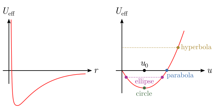
\[U_\text{eff}(u) = u\left(\frac{L^2}{2m}u -GMm\right).\]

This is quadratic, and quadratic potentials are easy: they lead to simple harmonic motion! The motion will be about the minimum of the potential, which occurs halfway between the two roots at

\[u_0 = \frac{GMm^2}{L^2}, \quad U_\text{eff}(u_0) = -\frac{1}{2}\left(\frac{GMm}{L}\right)^2.\]

Effective potentials work as follows. If the planet has total energy $E$, then

\[E = K + U_{\text{eff}}(u), \quad K = \frac{1}{2}m \left(\frac{du}{d\tau}\right)^2,\]

where $K$ is the linear kinetic energy, and $\tau$ is the relevant time variable for the $u$ coordinate. Somewhat subtly, this is not the same as the regular time $t$. If we want to interpret $K$ as the linear kinetic energy for the planet in $r$ coordinates as well, we must have the relation

\[\left|\frac{dr}{dt}\right| = \left|\frac{du}{d\tau}\right| \quad \Longrightarrow \quad \frac{1}{r^2}\frac{dr}{d\tau} = \frac{dr}{dt},\]

using $u = 1/r$. Here, we can sneakily use conservation of momentum again! Recall from above that $L\, dt = m r^2\, d\theta$. Thus, we can immediately solve for the time variable in $u$ coordinates:

\[r^2 \, d\tau = dt \quad \Longrightarrow \quad \tau = \frac{m}{L} \theta.\]

In other words, time in $u$ coordinates is proportional to angle! Finally, let’s determine the motion in $u$ coordinates. The “stiffness” $k$ of the restoring force, and hence angular frequency $\Omega$, are given by

\[k = U''_\text{eff}(u) = \frac{L^2}{m}, \quad \Omega = \sqrt{\frac{k}{m}} = \frac{L}{m}.\]

If we fix $E$, then the planet will oscillate around $u_0$ with some amplitude $A$, according to

\[u - u_0 = A \cos(\Omega \tau) = A \cos(\theta).\]

This is an ellipse with a focus at $u = \infty$.

Ellipses and eccentricities

In case you don’t believe me, let’s rewrite the harmonic motion in terms of $r$:

\[r = \frac{u_0^{-1}}{1 + A u_0^{-1} \cos(\theta)}.\]

This is the equation for an ellipse of eccentricity $\varepsilon = A u_0^{-1}$ and “semi-lattice rectum” $p = u_0^{-1}$, with a focus at $r = 0$, i.e. $u = \infty$. There are many things we could check here, but a good start is the relation between eccentricity and energy $E$. We have

\[0 = U_\text{eff}(u) - E = (u-u_0)^2 - u_0^2 - E.\]

The amplitude is simply the distance between the $u_0$ and the roots,

\[A = \sqrt{u_0^2 + E}.\]

A circular orbit has $A = 0$ and $r = 1/u_0$, which implies energy $E = -u_0^2$. We can check this energy is correct, since

\[E = \frac{L^2}{2m}\cdot u_0^2 - GMm u_0 = -u_0^2.\]

Since orbits are bound, i.e. have negative total energy, we expect they will cease at $E = 0$, or $A = u_0$. If we plug this into the eccentricity, we find

\[\varepsilon = A u_0^{-1} = 1,\]

which is the eccentricity of a parabola, so the orbit is indeed unbound. For strictly positive energies, we have hyperbolic orbits, $\varepsilon > 1$. It all hangs together!

The third law

We’ll do one more sanity check: Kepler’s third law. There is a trick to doing this. There is also a direct method where one simply evaluates an integral for $T$:

\[T = \int_0^{2\pi} d\theta\, \frac{dt}{d\theta} = \frac{m}{L}\int_0^{2\pi} d\theta\, r^2 = \frac{2mA}{L},\]

where $A$ is the area of the ellipse, using our earlier result for area, $2\, dA = r^2 \,d\theta$. Now, at this point, if you know about ellipses, you might remember that $A = \pi ab$, for the semi-major axis $a$ and semi-minor axis $b$. Thus, the period has the form

\[T = \frac{2\pi m ab}{L} \propto \sqrt{u_0} ab.\]

You might also know that the semi-major and semi-minor axis are related by $au_0^{-1} = b^2$, and hence $T \propto a^{3/2}$. This is Kepler’s third law! But suppose you don’t have all these facts at your fingertips. You can actually explicitly calculate the integral for $T$ (using for instance the residue calculus from complex analysis, or a table, or a symbolic algebra package), and directly get

\[T = \frac{m}{L}\int_0^{2\pi} d\theta\, \frac{u_0^{-2}}{[1 + A u_0^{-1} \cos(\theta)]^2} = \frac{2\pi}{\sqrt{GM}}\left[\frac{1}{u_0(1-A^2u_0^{-1})}\right]^{3/2} \propto a^{3/2}.\]

No geometry required! But if you’re more comfortable with ellipses, you can use them to evaluate a tricky integral.

Conclusion

Put simply, the effective potential is quadratic in $u = 1/r$, and all the conic sections arise from simple harmonic motion. This includes elliptical orbits, which wobble back and forth, and the parabolic and hyperbolic “orbits” which hit $u = 0$, i.e. go off to infinity in the $r$ coordinate. Although the $u= 1/r$ transformation is well-known — there is nothing new orbiting the sun — I haven’t found anything which emphasizes the simple harmonic motion. So hopefully there is some small novelty in presentation!