A hacker's guide to the Chandrasekhar limit
April 6, 2020. If you throw too many electrons into a box, it collapses under its own weight to form a black hole. But how many is too many? We will hack our way towards an order-of-magnitude estimate, and comment on the implications for astrophysics.
Contents
1. Introduction
Though they differ in size by many orders of magnitude, solar system and atom are superficially not so different. Both involve smaller bodies (electrons/planets) orbiting a much larger body (nucleus/sun) under the influence of a central force (electrostatics/gravity). Orbits also have finite occupancy. Part of the definition of a planet is that it “clears its neighbourhood” of any interlopers (sic transit gloria Pluto). Electrons automatically clear their orbitals by the Pauli exclusion principle, a point we will return to below.
But that’s where the resemblance ends. The solar system is classical, and planets can orbit the sun at any old radius they like. In contrast, atoms obey quantum mechanics, and the orbits are quantised, occuring only at certain allowed values. Quantisation has deep consequences for atomic structure, hence chemistry, hence life itself. We’re made out of exploded stars, sure, but biology is also quantum mechanics writ large.
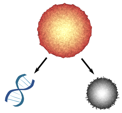
What about the stuff left behind? Once the outer layer of a star burns off, the leftover fuel is squished together by gravity to form a compact remnant or even a black hole. Most stars will turn into a remnant called a white dwarf. White dwarfs form a different link between stars and atoms, since like atoms, they are governed by quantisation. With some dimensional analysis, we can obtain an order-of-magnitude bound on the mass of white dwarfs called the Chandrasekhar limit, after Subrahmanyan Chandrasekhar, who derived it (much more carefully!) in 1931. It is the mass at which a white dwarf collapses to form a black hole.
Outline. We’ll start with Bohr’s model of the hydrogen atom and the quantisation of orbits, and then apply these ideas to a Fermi gas of non-interacting electrons on a circle. Even when the gas is at zero temperature, the Pauli exclusion principle creates an effective repulsion called degeneracy pressure. Stapling three circles together, we get a simple but accurate model of degeneracy pressure in stellar remnants. We find the Chandraskhar limit by determining when gravity beats degeneracy pressure. As a bonus, we also find the relation between white dwarf mass and radius.
Prerequisites. This post is aimed at high school students with an interest and background in physics. We assume basic Newtonian mechanics (kinetic energy and momentum) and the law of gravitation. Some familiarity with “old school” quantum mechanics (the Bohr model and de Broglie wavelength) is helpful, though we introduce the required concepts here, albeit briefly. On the math side, we use vector notation and need to know how to calculate a vector’s length.
2. Fermi gas
We’re going to consider a simple caricature of quantum mechanics, given by three rules:
- There is a set of allowed energies, $E_1 \leq E _2 \leq E_3 \leq \cdots$, a particle can have.
- Only one particle can occupy an energy level at a time.
- If we add particles, they occupy the lowest available energy level.
I think of this as the “hotel” model, since the quantum system is like a hotel with rooms costing $E_1\leq E_2 \leq \cdots$. Particles travel alone, and stay by themselves. Finally, particles are cheap, looking for the most affordable room the hotel can offer. None of these rules is true in general, so let’s spell out what systems it applies to.
The first rule states that energies don’t change when particles join the system, which is only true if the particles don’t interact. If particles repel each other and will pay more money to stay apart, or are attracted and will pay more money to be close, the hotel should change its prices! Physicists use the term “gas” for any weakly interacting collection of particles, so our rules describes a quantum gas.
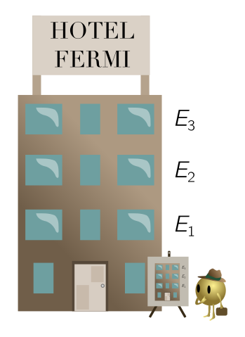
The second rule is the Pauli exclusion principle. This holds for electrons, and in fact, a much larger class of particles called fermions, which includes protons and neutrons. Our model describes a gas of fermions, or Fermi gas for short. The final rule — particles are as stingy as possible — means the gas is at zero temperature. At finite temperature, there is some chance arriving particles will splash out on a more expensive room! Our three rules describe Hotel Fermi, aka a zero temperature Fermi gas.
2.1. Bohr’s model
We’ll start by recalling Bohr’s model of hydrogen and the role played by quantisation. Bohr thought of the nucleus as a big, immovable positive charge, and the electron as a tiny orbiting negative charge. To explain why hydrogen emits and absorbs only certain colours of light, Bohr postulated that only certain orbits were allowed, satisfying the quantisation of angular momentum:
\[m_ev r = n \hbar, \quad n = 1, 2, 3, \ldots\]where the “quantum” of angular momentum is Planck’s (reduced) constant $\hbar$, and $m_e$ is the mass of the electron. There is a nice way of reformulating this using de Broglie’s notion of matter waves.
Let’s turn for a moment to light. The energy, momentum, and wavelength of a single photon of light can be written
\[E = \hbar \omega, \quad p = \frac{E}{c}, \quad \lambda = \frac{2\pi c}{\omega},\]where $\omega$ is the angular frequency of light and $c$ is its speed. Rearranging, one finds momentum and wavelength are related by
\[\lambda = \frac{2\pi c}{\omega} = \frac{2\pi \hbar}{p}.\]By analogy, de Broglie guessed that a massive particle could also exhibit wave-like behaviour, with a wavelength related to its momentum in the same way:
\[\lambda = \frac{2\pi \hbar}{p}.\]Plugging this into Bohr’s quantisation condition gives
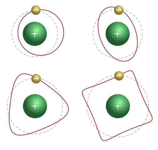
\[pr = n\hbar \quad \Longrightarrow \quad \lambda_n = \frac{2\pi r}{n}, \quad n = 1, 2, 3, \ldots.\]This has a lovely interpretation: since $2\pi r$ is just the circumference of the circle, the allowed orbits are those for which the matter wave is periodic, meeting up with itself after $n$ periods. The matter wave “fits”.
To connect to our “hotel” model of quantum mechanics, we need to find the energy levels for the electron. First, we can express kinetic energy in terms of momentum, hence in terms of de Broglie wavelength:
\[E_n = \frac{1}{2}m_e v^2 = \frac{(m_ev)^2}{2m_e} = \frac{p^2}{2m_e} = \frac{2\pi^2 \hbar^2 n^2}{m_e (2\pi r_n)^2}. \tag{1} \label{bohr-E}\]We still don’t know the radius of the orbit $r_n$, and we won’t need it below. However, the interested reader can supply it themselves in the following exercise.
Exercise 1. The key fact we haven’t used about the hydrogen atom is that the electron orbits due to electrostatic attraction. The attractive force between charge $q_1$ and $q_2$ is governed by Coloumb’s law, an inverse square law analogous to gravity:
\[F = \frac{k_eq_1q_2}{r^2},\]where $k_e$ is a constant analogous to $G$ in Newton’s law of gravitation.
(a) Show that the electron is pulled inward with force
\[F = \frac{k_e e^2}{r^2}.\](b) For an electron in a circle, the centripetal acceleration $a = v^2/r$. Use this and part (a) to derive the relation
\[p^2 = \frac{k_e m_e e^2}{r}.\](c) Use (b) to show that the orbits gets larger quadratically with $n$:
\[r_n = \left(\frac{\hbar^2}{k_e m_e e^2}\right) n^2.\](d) Conclude that hydrogen has energy levels
\[E_n = -\frac{p_n^2}{2m_e} = -\left(\frac{m_ek_e^2 e^4}{2\hbar^2}\right) \frac{1}{n^2}.\]Notice the minus sign in $E_n$. If we don’t add it, energy decreases with $n$. From Rule 3, electrons occupy the lowest available state, so they will zip off to infinity!
(e) For an ion with $Z$ protons in the nucleus, repeat the argument above to obtain the single-electron energy levels
\[E_n = -\left(\frac{m_ek_e^2 e^4}{2\hbar^2}\right) \frac{Z^2}{n^2}\]2.2. Electrons on a circle
You might hope that an atom is like the hotels described above, with energy levels (\ref{bohr-E}). But for better or worse, there is more to atomic physics than a few lines of algebra. Electrons interact, and keeping track of orbits in a multi-electron system is a finicky business. Rather than delving into these complexities, we will streamline the Bohr model.
We make two simplifying assumptions: first, take electrons to be non-interacting; second, fix a single orbit, of circumference $L = 2\pi r$. Then the Bohr-de Broglie quantisation condition becomes
\[\lambda_n = \frac{L}{n},\]and the energy levels (\ref{bohr-E}) become
\[E_n = \left(\frac{2\pi^2 \hbar^2 }{m_e L^2}\right) n^2. \tag{2}\label{circle-E}\]The proton is no longer required, since its only role earlier was to determine the orbital radius $r_n$, and we have fixed $r_n = r$ by fiat. (Since the electrons are no longer bound, this eliminates the minus sign we needed in Exercise 1.)
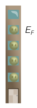
Suppose we throw $N$ particles onto the circle. The highest occupied energy level is called the Fermi energy $E_F$ (see Exercise 2). The fact that the Fermi energy is not just the lowest energy level has interesting consequences. The best way to think of temperature is in terms of its relation to average energy per particle:
\[E_\text{avg} \sim k_BT,\]where $k_B$ is Boltzmann’s constant. This suggests that, even though our Fermi gas is supposed to be at zero temperature, there is an “effective temperature” due to quantum effects. For lack of imagination, we call this the Fermi temperature, and define it by
\[T_F = \frac{E_F}{k_B}.\]Finally, in an ideal gas, temperature and pressure are related by the ideal gas law, $PV = N k_B T$. The fact that electrons are spread across energy levels can be viewed as an “effective pressure” $P_F$ due to quantum effects. This is also called degeneracy pressure. You can show in Exercise 2 that the degeneracy pressure for a circle is roughly
\[P_F \sim \frac{N E_F}{L}.\]We haven’t defined $P_F$ carefully, so this expression is only true to an order of magnitude, as indicated by the $\sim$ symbol.
Exercise 2. Let’s calculate some simple properties of the Fermi gas on the circle.
(a) Show that if we put $N$ electrons on the circle, the Fermi energy is
\[E_F = \left(\frac{2\pi^2 \hbar^2 }{m_e L^2}\right)N^2.\](b) By identifying $T = T_F$ in the ideal gas law, argue that
\[P_F \sim \frac{\hbar^2 N^3}{m_e L^3}.\]2.3. Electrons on a donut
A circle is nice and simple; too simple, in fact, to capture the physics of a real star. A star is a three-dimensional object, so we will need to upgrade our Fermi gas from a one-dimensional circle to something with three dimensions. This is one of the few cases where modelling our problem as a sphere in a vacuum is a bad idea! Quantisation on a sphere is complicated, which is part of the reason that deriving chemistry from physics is a tricky business.
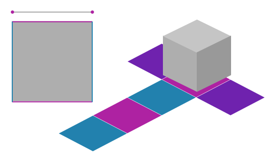
To avoid this difficulty, we will crudely approximate a sphere as three circles stapled together, with each circle associated to a different dimension. The result is a three-dimensional donut, so really, we are effectively modelling a star as a donut in a vacuum! To see how circles and donuts are related, we need to think about the circle a little differently. As a warm-up, we’ll show that stapling two circles gives a regular donut. (A similar approach is to start with quantisation on a line rather than a circle, then staple three lines to get a box, but our approach jives better with the hydrogen atom.)
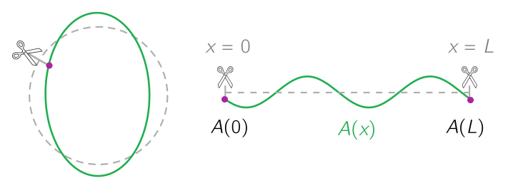
Take a circle of circumference $L$ and snip it at some point. Straightening out, we get a line of length $L$. According to Bohr-de Broglie, matter waves on the circle join smoothly at the point we snipped. Let $x$ be the coordinate on the line, with the “snip” at $x = 0$ and $x = L$. If $A(x)$ the amplitude of a matter wave, then
\[A(0) = A(L).\]To get the circle back, we can just glue the endpoints at $x = 0, L$.
We are now going to “square the circle”: lay two snipped circles at right angles, forming a square with horizontal coordinate $x$ (associated to one circle) and vertical coordinate $y$ (associated to the other). A wave is now a wobbly sheet drawn over the top of the square. But the left and right are identified, because we have a circle in the horizontal direction, and gluing the left and right of the square gives a cylinder. But the top and bottom are also identified, since we have a circle in the vertical direction. Gluing the two ends of the cylinder, we get a donut!
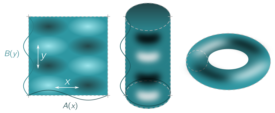
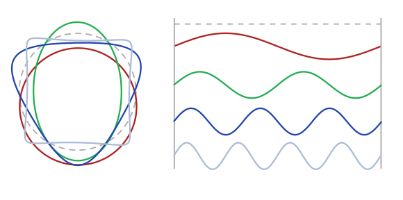
Quantisation on the donut is simple. Suppose a wave wobbles independently in the $x$ and $y$ directions, with wavelengths $\lambda_x$ and $\lambda_y$. We can impose the Bohr-de Broglie condition in each direction independently, so
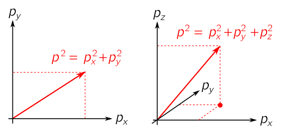
\[\lambda_x = \frac{L}{n_x}, \quad \lambda_y = \frac{L}{n_y}.\]In the image above, for instance, we have $n_x = 1$ and $n_y = 2$, so $\lambda_x = L$ and $\lambda_y = L/2$. To determine the energy, we use the fact that $p^2 = |\vec{p}|^2$ is the squared length of the momentum vector, $\vec{p} = (p_x, p_y)$:
\[p^2 = p_x^2 + p_y^2.\]This is just Pythagoras’ theorem applied to momentum. (We depict momentum vectors in two and three dimensions below.) Finally, the de Broglie relation in each direction gives $\lambda_x = 2\pi\hbar/p_x$, $\lambda_y = 2\pi\hbar/p_y$, hence
\[E_{n_x, n_y} = \frac{p^2}{2m_e} = \frac{p_x^2 + p_y^2}{2m_e} = \left(\frac{2\pi^2 \hbar^2 }{m_e L^2}\right) (n_x^2 + n_y^2).\]We can assemble the two integers or mode numbers $n_x, n_y$ into a mode vector $\vec{n} = (n_x, n_y)$, so
\[p^2 = \left(\frac{2\pi\hbar}{L}\right)^2 |\vec{n}|^2.\]We can perform exactly the same trick for even more circles. In particular, to get a three-dimensional example, let’s take a product of three circles of length $L$. We can view this as a cube of side length $L$ with periodic boundary conditions, or alternatively, a three-dimensional donut. Pythagoras’ theorem (applied twice) gives $p^2 = p_x^2 + p_y^2 + p_z^2$.
If the wavelengths in each direction are $\lambda_x = L/n_x$, $\lambda_y = L/n_y$, and $\lambda_z = L/n_z$, with corresponding mode vector $\vec{n} = (n_x, n_y, n_z)$, we can repeat our reasoning for the donut to obtain the expression for $E_{\vec{n}}$:
\[E_{\vec{n}} = \left(\frac{2\pi^2 \hbar^2 }{m_e L^2}\right) |\vec{n}|^2 = \left(\frac{2\pi^2 \hbar^2 }{m_e L^2}\right) (n_x^2 + n_y^2 + n_z^2).\]We end with a bit of terminology we will use below. A circle is a periodic line (opposite ends glued), and a donut is a periodic square (opposite sides glued). Similarly, we can view a three-dimensional donut as a periodic cube (opposite faces glued).
We can generalise this to higher-dimensional donuts, but three dimensions will be sufficient for our purposes!
Exercise 3. Let’s get a feeling for energy levels on a (two-dimensional) donut.
(a) Compute the lowest three energy levels, and sketch them on the square.
(b) If I put $N = 10$ electrons in the donut, what is the Fermi energy?
2.4. Approximating the Fermi sea
The Fermi sea is the set of occupied energy levels for a Fermi gas. In the hotel analogy, it’s just the set of occupied rooms! As Exercise 3 demonstrates, filling out the Fermi sea on a donut takes some work. It is even trickier to calculate energy levels on the three-dimensional donut, where we need to consider all the different possibilities for $\vec{n} = (n_x, n_y, n_z)$. Calculating the Fermi energy $E_F$ for large $N$ seems like a hard combinatorics problem best suited to a computer.
Thankfully, there is a neat shortcut for filling out the Fermi sea when $N$ is large. We’ll do the calculation for a regular donut, and leave the three-dimensional donut to Exercise 4. For the donut, the mode vectors $\vec{n} = (n_x, n_y)$ live on a Cartesian plane, with one point per unit area. If we draw a circle of radius $n_F$ in this plane, centred at the origin, the number of points it contains is approximately equal to the area:
\[N \approx \pi n_F^2.\]This approximation gets better as $n_F$ gets larger, as illustrated in the picture below.
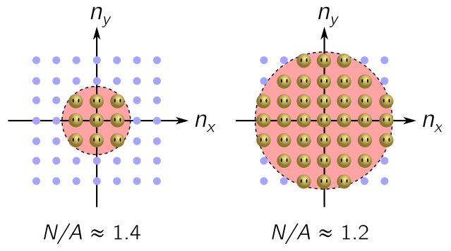
The maximum length of a vector in this disk is $|\vec{n}|^2 \approx n_F^2$, and the disk contains all vectors of smaller length as well. Electrons added to the system will find the shortest available vector, filling out the disk radially. We learn that for large $N$, the Fermi energy is
\[E_F \approx \left(\frac{2\pi^2 \hbar^2 }{m_e L^2}\right) n_F^2 \approx \left(\frac{2\pi \hbar^2}{m_e L^2}\right) N.\]For a handful of matter, say $N \sim 10^{23}$ electrons, this approximation is more or less perfect. On a donut, the degeneracy pressure is calculated as above, but $L$ is replaced by $L^2$, since this was the volume of the system in the ideal gas law. This gives
\[P_F \sim \frac{NE_F}{L^2} \sim \frac{\hbar^2 N^2}{m_e L^4}.\]It’s your turn now!
Exercise 4. Consider a Fermi gas in a three-dimensional donut.
(a) For $n_F \gg 1$, show that a ball of radius $n_F$ in $\vec{n}$-space contains $N \approx 4\pi n_F^3/3$ points.
(b) Argue that for large $N$, the Fermi energy is
\[E_F \approx \left(\frac{2\pi^2 \hbar^2}{m_eL^2}\right) \left(\frac{3N}{4\pi}\right)^{2/3}.\](c) Conclude that the degeneracy pressure is
\[P_F \sim \frac{\hbar^2 N^{5/3}}{m_e L^5}.\]3. Adding gravity
We’re almost ready to perform our thought experiment of throwing electrons into a box until we make a black hole. But to apply our Fermi gas model to old stars, we need to learn a little astrophysics.
3.1. Ultrarelativity
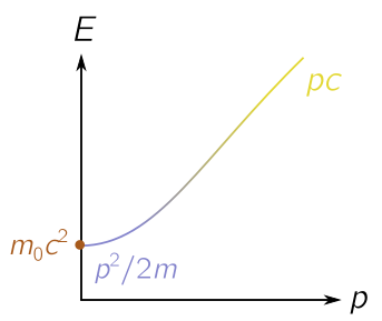
The gravitational force is strong with stars, particularly old stars who have shed their outer layers and contracted to a dense core. This means most particles are zipping around at close to the speed of light, and the earlier, Newtonian form of kinetic energy we used is no longer appropriate. Instead, we have to use relativity! Recall Einstein’s famous equation $E = mc^2$. Note that it can be written in the slightly more transparent form
\[E^2 = (m_0 c^2)^2 + p^2 c^2,\]where $p^2 = |\vec{p}|^2$ is the momentum squared as usual, and $m_0$ is the mass of the particle at rest. (The usual $m$ is relativistic mass, which changes with speed.) Particles in an old star usually have much more momentum than rest mass, so the kinetic energy takes the ultrarelativistic form:
\[E^2 \approx p^2 c^2 \quad \Longrightarrow \quad E \approx |\vec{p}|c.\]We can picture the different regimes below.
All the business about Bohr-de Broglie quantisation remains unchanged, and in fact the analogy to light is much improved! It follows that
\[E_{\vec{n}} = \frac{2\pi\hbar c|\vec{n}|}{L}.\]I’ll let you find the degeneracy pressure in Exercise 5.
Exercise 5. Consider an ultrarelativistic Fermi gas in a periodic cube of volume $V$. Show that, for $N \gg 1$, the degeneracy pressure is
\[P_F \sim \hbar c\left(\frac{ N}{V}\right)^{4/3}.\]3.2. White dwarfs and neutron stars
Above, I referred mysteriously to various stellar remnants. Let’s see what these remnants are, and how they are related to the Fermi gas we’ve been discussing. It will be useful to weigh stars using the mass of our sun,
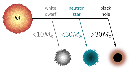
\[M_\odot = 2\times 10^{30} \text{ kg}.\]Very briefly, stars fuse hydrogen into helium, and so on into the heavier elements. The pressure generated by these thermonuclear reactions allows the star to resist its own gravity. But once a star runs low on fuel, gravity begins to win, and the fate of the star depends on its mass $M$ before collapse. There are three possible endpoints:
- White dwarf. If the star weighs less than $10$ suns ($M < 10 M_\odot$), it will contract until the degeneracy pressure of the electrons in unspent nuclear fuel stops the collapse. This is the fate of most stars in the universe.
- Neutron star. If the star is between $10$ and $30$ solar masses ($10 M_\odot < M < 30 M_\odot$), electron degeneracy pressure is not enough, and a more desparate gambit is required. Electrons and protons combine to make neutrons, and neutron degeneracy pressure plus repulsion due to the strong nuclear force arrests gravitational collapse.
- Black holes. If the star is heavier than $30$ suns ($30 M_\odot < M$), nothing can resist gravity, and it ineluctably collapses to form a black hole.
We’ll focus on white dwarfs here, but neutron stars and black holes will also make important appearances.
The core of a white dwarf is electrically neutral, consisting of $N$ electrons and $N$ protons. Since protons are much heavier than electrons, they provide most of the star’s mass. Overall neutrality means that electrostatic repulsion plays a small role, and the degeneracy pressure of the electrons dominates. Assuming gravity is strong and the electrons are ultrarelativistic, we might hope the degeneracy pressure is
\[P_F \sim \hbar c\left(\frac{ N}{V}\right)^{4/3}\]where $V$ is the volume of the white dwarf. This expression is based two assumptions which don’t seem to hold here: the gas is at zero temperature, and contained in a three-dimensional donut. Luckily, neither of these is a problem.
- Temperature. We can approximate a Fermi gas as zero temperature provided $T$ is much smaller than the Fermi temperature, $T \ll T_F$. White dwarfs are typically around $T = 10^7 \text{ K}$, while the Fermi temperature is order $T_F \sim 10^9 \text{ K}$ (Exercise 6).
- Shape. A white dwarf is a sphere not a three-dimensional donut. Nevertheless, our model works because sphere and donut are just different choices of boundary condition, and as $N$ gets large, boundary conditions become irrelevant.
Thus, our expression of $P_F$ should apply (approximately) to a real-life white dwarf.
Exercise 6. A white dwarf the size of the earth has a density around $10^9 \text{ kg/m}^3$, consisting mostly of protons. Show that the Fermi temperature is $T_F \sim 10^9 \text{ K}$.
Hint. Use the ideal has law to relate $P_F$ and $T_F$. The proton mass $m_p$, speed of light $c$, Planck’s constant $\hbar$, and Boltzmann’s constant $k_B$ are given below:
\[\begin{align*} m_p & = 1.7 \times 10^{-27} \text{ kg} \\ c & = 3.0 \times 10^8 \text{ m/s} \\ \hbar & = 1.1 \times 10^{-34} \text{ J} \cdot \text{s} \\ k_B & = 1.4\times 10^{-23} \text{ m}^2\text{ kg}/\text{ K s}^2. \end{align*}\]You can check the claim about density in Exercise 9.
3.3. The Chandrasekhar limit
We’re finally ready to calculate the mass of the largest white dwarfs, called the Chandrasekhar limit. Our goal will be to calculate the “self-pressure” on the white dwarf due to gravity, and compare to the degeneracy pressure. Recall Newton’s law of gravitation,
\[F = \frac{GMm}{R^2}\]where $M,m$ are separated by $R$, and $G = 6.7\times 10^{-11} \text{ m}^3/\text{kg s}^2$ is Newton’s constant.
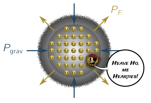
Consider a spherical white dwarf of mass $M$ and radius $R$. What gravitational force does this exert on itself? Obviously a precise answer will depend on the composition of the dwarf and other details, but we can make an order-of-magnitude estimate from dimensional analysis. In Newton’s law, we set both masses equal to $M$, since the white dwarf is both doing the pulling and experiencing the pull. Similarly, the only length scale in the problem is the radius $R$, so we guess
\[F_\text{grav} \sim \frac{GM^2}{R^2}.\]Since pressure is force divided by area, the gravitational self-pressure is going to be this force divided by the surface area of the sphere, or
\[P_\text{grav} \sim \frac{F_\text{grav}}{A} \sim \frac{GM^2}{R^4}.\]Finally, we can calculate the Chandrasekhar limit. The mass of a white dwarf is mostly protons, with $M = Nm_p$, while $V \sim R^3$. Thus, we can write the degeneracy pressure as
\[P_F \sim \hbar c \left(\frac{N}{V}\right)^{4/3} \sim \hbar c \cdot \frac{(M/m_p)^{4/3}}{R^4}.\]Let’s set this equal to the gravitational self-pressure, $P_\text{grav} = P_F$, and solve for the mass:
\[\begin{align*} \frac{F_\text{grav}}{A} \sim \frac{GM^2}{R^4} & \sim \hbar c \cdot \frac{(M/m_p)^{4/3}}{R^4} \\ \Longrightarrow \quad M^{2-4/3} = M^{2/3}& \sim \frac{\hbar c}{G} \frac{1}{m_p^{4/3}}. \end{align*}\]Raising both sides to the power $3/2$, we obtain Chandraskehar’s famous bound:
\[M_C \sim \left(\frac{c\hbar}{G}\right)^{3/2}\frac{1}{m_p^2}.\]In 1983, Chandra won the Nobel Prize in Physics, largely for his work on white dwarfs.
Although we have reached our main goal, the exercises below convert Chandrasekhar’s limit to solar masses (Exercise 7), throw electrons into a box until it collapses (Exercise 8), deduce the mass-radius relation for non-relativistic white dwarfs (Exercise 9), and finally, explore two-dimensional stellar remnants (Exercise 10). Have fun!
Exercise 7. Evaluate $M_C$ numerically and compare to the mass of the sun. You should find
\[M_C \sim\, 1.7 M_\odot.\]The state-of-the-art limit, incorporating details about the white dwarf’s composition and structure, is $ M_C \approx 1.44 \,M_\odot$. We’ve done remarkably well!
⁂
Exercise 8. Let’s finally solve the problem of how many electrons you can plonk into a box before it forms a black hole. (The difference from the white dwarf is that there are no protons.)
(a) Argue that, if the electrons are ultrarelativistic, the box of electrons will collapse once the mass reaches
\[M_\text{box} \sim M_C \left(\frac{m_p}{m_e}\right)^2 \approx 5 \times 10^7 \, M_\odot.\]This is so ridiculously heavy that it would form a supermassive black hole, like the ones found at the centre of the Milky Way and other galaxies.
(b) Calculate $N_\text{box}$, the number of electrons in the box.
⁂
Exercise 9. We can repeat our pressure-balancing argument with the non-relativistic Fermi gas. This is appropriate to smaller and less gravitationally extreme white dwarfs.
(a) Recall the non-relativistic degeneracy pressure,
\[P_F \sim \frac{\hbar^2 }{m_e}\left(\frac{N}{V}\right)^{5/3}.\]Compare to gravitational self-pressure, and show that in equilibrium,
\[R \sim \left(\frac{\hbar^2}{m_e m_p^{5/3}G}\right)M^{-1/3}.\]This mass-radius relationship tells us that the white dwarf shrinks as it gets heavier!
(b) Compute the mass density of a white dwarf the same size as the earth, assuming we are in the non-relativistic regime. The earth has radius $R = 6.4 \times 10^6 \text{ m}$, while an electron has mass $m_e = 9.1 \times 10^{-31} \text{ kg}$. You should obtain
\[\rho \sim 5 \times 10^{9} \text{ kg/m}^3.\]This is very dense: a single cubic metre weighs as much as five Empire State Buildings!
⁂
Exercise 10. Consider a two-dimensional white dwarf. Gravity in two dimensions obeys a modified version of Newton’s law:
\[F = \frac{G_{(2)} Mm}{R},\]where $G_{(2)}$ is a modified constant. Is there a Chandrasekhar limit? If so, what is it?
3.4. Neutron stars
How are neutron stars different from white dwarfs? Neutrons are fermions, so if we pack them into a box, there will be degeneracy pressure as before. Neutron stars are still cold compared to the Fermi temperature, so the zero-temperature approximation is good. If we repeat the reasoning above, balancing neutron degeneracy pressure against gravitational self-pressure, we find
\[M_N \sim \left(\frac{c\hbar}{G}\right)^{3/2}\frac{1}{m_n^2} \approx 1.7 \, M_\odot\]once more, since a neutron has almost the same mass as a proton, $m_n \approx m_p$. It seems like the Chandrasekhar limit should also apply to neutron stars.
But there is a subtlety we did not include: the strong nuclear repulsion between neutrons. This repulsion is poorly understood and difficult to model, but the analogue of the Chandrasekhar limit for neutron stars is called the Tolman-Oppenheimer-Volkoff (TOV) limit, mainly based on numerical simulations. These simulations suggest that nuclear repulsion is comparable in strength to neutron degeneracy, with
\[M_\text{TOV} \approx 2.17 \, M_\odot.\]To an order of magnitude, our naive guess agrees with the state-of-the-art!
4. Conclusion
If we take Bohr’s model of the atom and strip away the complexities of different orbits and interacting electrons, we end up with a single orbit on which we can put as many electrons as we like. Doing this three times gives a surprisingly good model of a white dwarf! The Pauli exclusion principle stops the white dwarf from collapsing under its own weight. But at the Chandrasekhar limit, gravity wins, and the white dwarf implodes into a black hole. The limit is also remarkably close to the best known bounds on neutron star mass, given that we ignored the strong force repulsion.
It’s amazing that we can simplify the hydrogen atom, and use it to learn about the death of stars. This is physics at its best: simple ideas with incredible power. And in the words of Chandra himself,
What is intelligible is also beautiful.
While a star’s ejecta may go on to form life, remarkable for its complexity, what is left behind is beautiful by virtue of its simplicity.