September 04, 2019. In the 21st century, mathematical skills are more important than ever before, but high school maths classes are dull, alienating and disempower students. How do we improve them, and plug some of the holes in the pipeline? I propose we make maths interesting! I illustrate the approach for teaching derivatives.

Contents

1. Introduction
   1. Stuck in the scrubland
   2. A patch of scrubland
   3. Shrubs and maximin
   4. Roads to nowhere
2. Views of the summit
   1. The mean value theorem
   2. A kink in the argument
   3. Slice of pi
3. Mining for patterns
   1. Sublime moth balls
   2. Irodov’s triangle
   3. Sand piles, slopes, and self-organisation
4. Miscellaneous issues
5. Conclusion

1. Introduction

The essence of mathematics lies precisely in its freedom.

In high school, I was one of those kids. I thought maths class was about as fun as watching paint dry, except that a fresh coat of paint might add colour to the world. I harboured no such illusions about mathematics. Would I use trigonometry on my tax returns? Or solve simultaneous equations for recreation? Finding $x$ was somebody else’s problem. I scraped by with passes, aping textbook examples and cramming for tests, but maths class was a particularly dull game, with rules I didn’t care about beyond the next quiz. The situation was so bad that, at age 15, I had to teach myself from scratch how to add fractions and multiply negative numbers. I had just never internalised those rules.

Taking philosophy a few years later, I encountered set theory for the first time and it blew my gourd. First of all, there was Bertrand Russell’s wonderful paradox about the set of all sets which don’t contain themselves. Is this big set a member of itself or not? If it is a member of itself, by definition it’s not a member of itself; and if it’s not a member of itself, by definition it is a member of itself. Neither can be true, so the big set can’t exist without breaking logic (i.e. generating a contradiction).

This is more than a novelty: Russell’s paradox can be jerry-rigged into an argument that there are different sorts of infinity! This is the sort of power that philosophers, using mere words, could only dream of. I saw that maths could be deep and bewitchingly strange.

At the same time, I was reading pop science books about fun topics like relativity, black holes and quantum mechanics. The books were mysterious but inviting, filled with pictures and metaphors and colourful examples that tantalised but did not, ultimately, enlighten. I began to suspect that I was missing something. To paraphrase Galileo, if I wanted to speak with the universe, it looked like I needed to learn its language, which was mathematics rather than colourful analogies. (See Brent Yorgey’s blog post on the temptation of analogies.) I switched from philosophy to maths and physics and never looked back.

I was lucky. Despite setting off in the opposite direction, I stumbled onto a hidden realm of extraordinary beauty and power. But how many students are unlucky? How many go through high school, numbed by repetition, cramming and copying just enough to pass tests, but never seeing that there’s a mathematical world out there which happens to exquisitely describe our world? The problem, I’ll argue, is that maths education is stuck in a sort of scrubland with no views into this enchanted realm.

1.1. Stuck in the scrubland

To make the problem more vivid, imagine a reality where, instead of maths, you were forced to take hiking classes in high school. Every day, you and your classmates would trudge through a barren, featureless scrubland, with no views, no peaks, and no apparent goal other than the hike itself. Whenever the class complained that the walk was boring or pointless (and who hikes in real life anyway?) the teacher would recite the dictum that walking was an important life skill. Heck, if you can’t walk, how do you expect to get a job! Privately, teach had to admit: two monotonous hours in the scrubland, every day for six years, did seem excessive, and they hated it too. But that’s just the way things were done.

Would you have enjoyed this hiking class? Or would you have lost interest and started lagging behind? Maybe, in time, you would have come to proudly identify as a bad hiker. The problem with these classes is clear. For most of us, walking is not an intrinsically interesting activity; there needs to be a motivation to walk, something to walk towards or to look at en route. That’s what hiking proper is all about. But if there’s no motivation, it becomes a chore, and rather than being trained to hike, you will be trained to avoid hiking.

Why have hiking classes anyway? Why don’t we ditch the hikes, and teach students how to walk to the corner store, the bus stop, or around the block with a dog in tow, the sort of walking most adults actually do? This would have made sense a hundred years ago. But let’s imagine that there’s now a whole sector of the economy which depends on advanced hiking skills, a need for wayfarers, explorers and hunters to meet the needs of society as a whole. We need hiking classes to act as an intake mechanism, drawing students into the field and equipping them to explore. And maybe we just want them to enjoy the natural world!

Some students seem to have a natural yen for walking. They can walk faster, and for longer distances; some hike outside of class, join the school club, and even do it competitively. Maybe we should channel our resources towards these “natural walkers” and let the rest opt out. But walking is a skill that can be developed, and most of these “natural walkers” are in fact motivated by non-scrubland experiences. Their parents took them out into nature, or they read about inspiring walks in a book with pictures, something like the pop science books I mentioned. They don’t visit the scrubland in their free time! These non-scrubland experiences, rather than natural ability, pushed them to develop their walking skills. There may be natural differences in ability, but they do not explain most variation in performance.

The fix is clear: we should stop marching students through the scrubland. Instead, we should guide them into varied and stimulating terrain, through forests, along canyons, and towards the strange rock formations in the distance. With time, they could learn to camp in the wilderness, explore uncharted wastes and conquer summits. I think interest would blossom in unexpected places. By going on real hikes, we would stop wasting student time, improve social outcomes by attracting more students into the hiking sector, and perhaps most importantly, show them that there’s a whole world out there, waiting to be relished and explored.

1.2. A patch of scrubland

The analogy to maths education and its shortcomings is fanciful but hopefully clear. Walking is the ability to manipulate symbols. Some people are naturally drawn to playing with symbols, some people aren’t. But maths is not symbol manipulation any more than hiking is walking! Manipulating symbols is how mathematics is done, but it’s not why we do it. And like walking, symbol manipulation is a skill that can be developed.

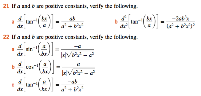
Then again, if you look at most high school textbooks, you could be forgiven for thinking otherwise. What should be a journey into the mathematical world is, in most cases, a joyless plod through a scrubland without context, without use, and without beauty. Here’s a patch of scrubland, courtesy of an anonymous Australian textbook:

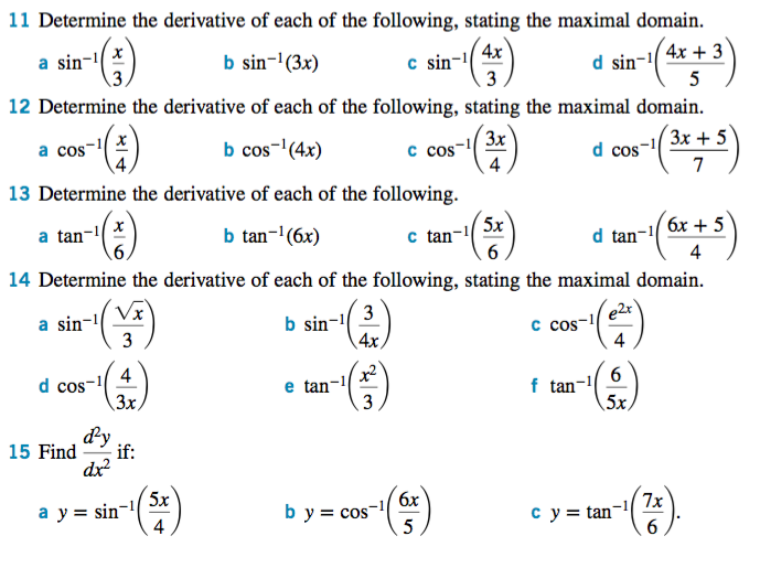
The topic is calculus, one the great milestones of Western thought. And here, we’re finding… rates of change of … some functions, I guess. What do these functions do? Why do I care? Who is inverse sine to me? These questions are unforgivably dull when there is literally hundreds of years of material to draw on. I wish I was cherry picking, but we will see below that the rest of the chapter is the same. This is what I mean by the scrubland: no landmarks, nothing for the eye to latch onto, just an endless plain of withered, ankle-high shrubs.

1.3. Shrubs and maximin

What makes these questions so bad? I propose that they fail the shrub test:

Would anyone bother to read this in their own time?

Would they read it if they didn’t have to pass a quiz? If not, you have shrubs, and shrubs kill interest. No one wants to spend hours looking at shrubs. If you force them to, you’re wasting their time and teaching them to avoid hiking.

The shrub test is a great start — and one that very few maths classes pass — but it’s still a low bar. All we ask is that somebody might conceivably read it for fun. And this leads to a different failure mode: when questions only appeal to a minority of students. This is part of the pedagogical “wisdom” behind the scrubland: write material which is uniformly unappealing so that nobody is left out. We can all share in the joy of shrubs!

How do we pass the shrub test but remain fair to students? I think we should borrow some ideas from political theory. American philosopher John Rawls was the 20th century’s pre-eminent theorist of fairness in the political context. Instead of using average utility (roughly, average personal good) as an organising social principle, he suggested something called the maximin rule: maximise the outcomes for those who are least well-off. From a game theory perspective, maximin (maximising the minimum outcome) is the right strategy when you can’t play the numbers due to extreme uncertainty. A secondary argument is that maximin should lead to a “trickle up” effect where everyone benefits.

Of the various tests we could adopt, I think there is a similar maximin test which should supersede the shrub test:

Would the least-engaged students bother to read this in their own time?

This is extremely stringent, but I think it’s right. Why? First of all, it’s fair. The students who are already involved and making progress have a basic level of a particular social good, engagement, that students on the margins don’t. It also seems plausible that by making class more interesting for the least-engaged, we make it more interesting for everyone, the “trickle up” effect Rawls thought applied to social goods generally. The best statistical evidence that it works is the JUMP method, pioneered by John Mighton.

A game-theoretic argument for the maximin test is the complexity of teaching. Besides the choice of material (which I’m emphasising here), there’s a whole host of other variables to consider, from pedagogy and lesson planning, demographics, classroom management, technology, and so on, all of which play a role in the effectiveness of a class. How do you optimise average student outcomes in this multidimensional landscape? It looks intractable for any class which isn’t also a research project. Given the uncertainties, game theory tells us we should focus on maximising the minimum outcome. I think the worst outcome is permanently turning students off mathematics and its sister sciences.

If we were hiking, the maximin test would translate into the simple requirement that we choose hikes even the students at the back of the group want to go on, and we don’t leave them behind. If interest, rather than inborn ability, determines success, then instead of marching slowly through featureless terrain, our best bet is to pick an exciting destination with diversions and enticements along the way.

1.4. Roads to nowhere

Students of hiking need practice before they can wander off into the foothills, armed only with a compass and a sense of adventure. Similarly, young mathematicians probably need to build their chops before they can do real maths. But if we show them where they’re headed, and all the amazing things they’ll be able to do when they get there, they won’t mind practicing. And this brings us to the real problem: not that students drill, but that the scrubland never ends. They drill in order to keep drilling. They study shrubs here, so they can classify some other shrubs down the road. Nobody is enlightened, empowered, or entertained. (I’ll discuss alternatives to drill below.)

The truth is that scrubland is easy for everyone but the students. You don’t need to be a good hiker to guide a class through the scrubland, and if you want to write a textbook, just fill it with lifeless, shrub-like variants of the same problem, sprinkled from that bag of shrub seeds you got at the nursery. The responsibility for getting us out of the scrubland doesn’t lie with teachers, or even textbook writers, but the people who write the curriculum. From their perspective, it’s much easier to maintain the scrubland than to chart a new course into the mathematical world. That takes time, money, and vision, and these are perennially in short supply.

But as in the hiking analogy, we don’t make mathematics compulsory for 10 years just to build up basic numeracy. This doesn’t match what we actually teach! Otherwise, why is geometry in the curriculum, logarithms, or combinatorics? These are not tools most adults have recourse to in their daily lives. Clearly, kicking around in the system is the assumption that mathematical thinking is valuable.

Even if we do not value it for its own sake, or the pleasure it brings, mathematical skills are essential to society as a whole. I’m not talking about the ability to calculate a tip or sniff out a dodgy lease-purchase scheme. I’m talking about dealing with the ongoing effects of climate change, big data, artificial intelligence, or personalised medicine, issues which call for explorers with higher-order hiking skills and a taste for the unknown. The stakes couldn’t be higher. Curriculum writers need to get out of their pickup trucks, drop their paintbrushes, and start talking to professional hikers, people who know the landscape and use the trails. Together, they can move mathematics out of the scrubland, and into the 21st century with all its challenges and complexities.

2. Views of the summit

I want to suggest two directions out of the scrubland. The first direction is pure mathematics, towards abstraction, generalisation, proof, and most importantly, beauty. Aesthetic considerations are famously important to pure mathematicians. The philosopher Bertrand Russell said that pure maths had a “beauty cold and austere, like that of sculpture”, and was “capable of a stern perfection such as only the greatest art can show”. (I think this underemphasises how much darn fun it is.) English mathematician G. H. Hardy elevated beauty to a requirement, stating that “beauty is the first test: there is no permanent place in the world for ugly mathematics.”

Sound like any high school maths class you ever took? It’s almost as if people got the Hardy quote backwards: there seems to be no permanent place in the classroom for beautiful mathematics. Let me show you what passes for pure mathematics in our advanced textbook:

This looks different from the earlier patch of scrubland until you notice these are more or less the same questions with letters replacing numbers. The shrubs are painted blue, but they are still shrubs.

Instead of dressing up shrubs, we should find a mountain to scale. Now, some mountains can only be scaled by professionals. But we don’t always need to scale a mountain to appreciate big peaks; with a bit of ingenuity, we can usually find a nearby hill with a gentler slope and a partial view of the summit. In pure mathematics, mountains are things like theorems (important proven results), conjectures (important unproven results), definitions and examples. “Important” means a variety of things, but as Hardy and Russell suggest, beauty is perhaps the principal criterion. Beauty in maths, as in art, is subjective, so we are left with the enviable task of choosing multiple beautiful things for students to look at. Hopefully one of them sticks!

Since we have spent a little time looking at calculus, I will illustrate how we can do this for derivatives: a neat little summit of generalisation called the mean value theorem; a monster dwelling in the badlands called the blancmange function; and finally, a much nobler use of inverse sine to provide a scheme for approximating $\pi$.

2.1. The mean value theorem

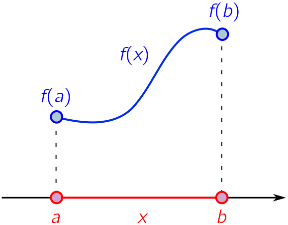
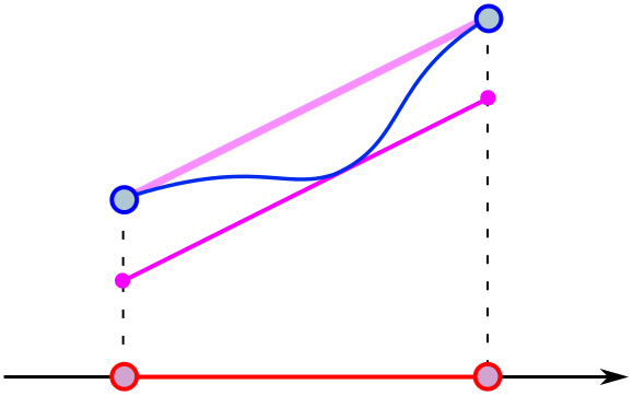
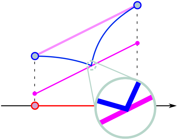
Our first example will be the mean value theorem (MVT). Instead of scaling the mountain and giving a fully rigorous proof, we will content ourselves with a good prospect from lower elevations using heuristics and visual aids. Suppose we have a continuous function $f(x)$ defined for $a \leq x \leq b$. This is pictured on the Cartesian plane below.

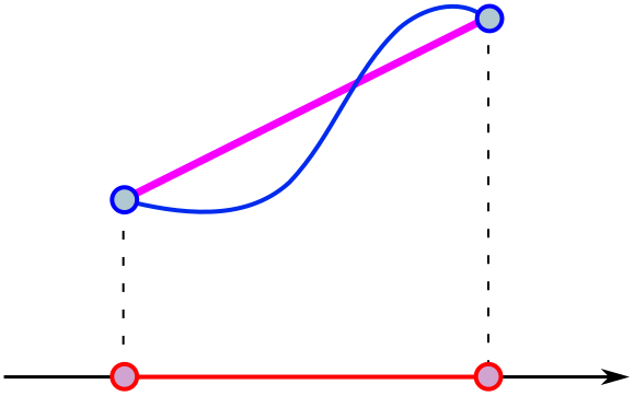
Now draw a line between the endpoints of the graph.

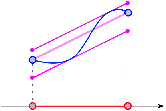
What happens if we shift the purple line (without tilting) up or down? In this example, there are two shifts where the line just touches (is tangent to) the curve.

Is it possible to draw a different graph so the purple line is tangent at one point? If you give students some time to experiment, they should find examples like the following:

What about no points where the graphs are tangent? With some time to play around, students should come to doubt that such curves exist. How can they prove it? One approach lies in the definition of “just touching”. Imagine zooming in infinitely close to the point of tangency, so the blue curve becomes straight (more or less what we mean by the derivative). You can convince students that the blue and purple lines must have the same slope at this point of intersection. If they had different slopes, they would cross each other rather than being tangent!

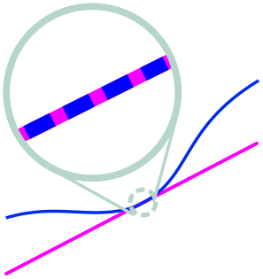
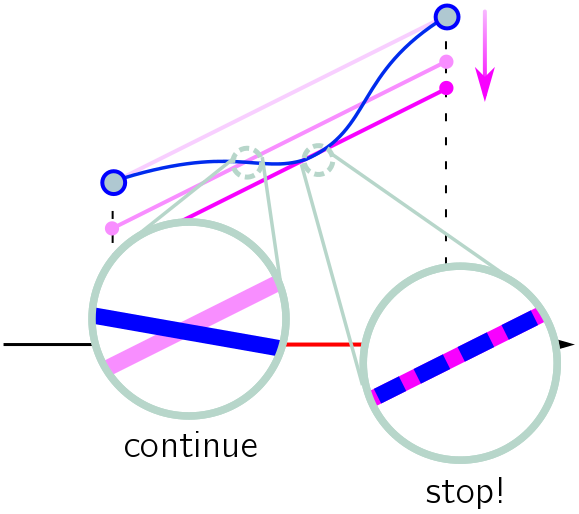
This suggests a visual proof, which students could discover for themselves with a little guidance. First of all, it’s clear that some of the blue curve should lie above the purple line, or below the purple line, otherwise it is the purple line and we have (infinitely) many points of tangency. But let’s assume that some of the blue curve lies below the original purple line. Now, move the purple line down until it can’t go further without missing the blue curve altogether. If the purple line wasn’t tangent to the blue at this extreme point, the blue would cross through the purple and we could continue moving it down. From our earlier discussion, this means they have to be tangent!

Since the purple line is straight, we can easily calculate its slope:

\[\text{slope} = \frac{\text{rise}}{\text{run}} = \frac{f(b)-f(a)}{b-a}.\]

For a function $f(x)$ on $a\leq x \leq b$, there is a point $c$ where the derivative equals the “mean” slope between its endpoints:

\[f'(c) = \frac{f(b)-f(a)}{b-a}.\]

This statement is the MVT! A nice feature of our proof is that (combined with root-finding methods) it can be turned into an algorithm for finding the point $c$. We didn’t need anything fancy, just some pictures and a solid feeling for what the definitions mean.

---

What can we do with this? One use of the MVT is to put intuitions about the sign of the derivative on firm footing:

• A continuous function $f: [a, b] \to \mathbb{R}$ with $f’ = 0$ on $(a,b)$ must be constant.
• A continuous function $f: [a, b] \to \mathbb{R}$ with $f’ > 0$ on $(a,b)$ is increasing.
• A continuous function $f: [a, b] \to \mathbb{R}$ with $f’ < 0$ on $(a,b)$ is decreasing.

Each of these statements can be proved by reductio ad absurdum: assume the consequent doesn’t hold, zoom in on a subinterval whose endpoints exhibit this failure, and apply the MVT. Let’s do the first one.

If $f’ = 0$ on $[a, b]$, but $f$ is not constant, then there is a subinterval $[a_1, b_1] \subseteq [a ,b]$, where $f$ assumes different values at either end, $f(a_1) \neq f(b_1)$. But applying the MVT to this subinterval shows that, at some point $c \in [a_1, b_1]$,

\[f'(c) = \frac{f(a_1)-f(b_1)}{a_1 - b_1} \neq 0.\]

This contradicts our assumption that $f’ = 0$ throughout $[a,b]$. Done!

---

It also leads to elegant, nontrivial inequalities about familiar functions. For instance,

\[|\tan^{-1}(x) - \tan^{-1}(y)| = \left|\frac{x - y}{c^2 + 1}\right| \leq |x - y|.\]

If we introduce contraction mappings (another conceptually simple and computationally tractable idea), we can turn this fact about inverse tan into a scheme for finding approximate solutions to transcendental equations like

\[x = 0.1 + \tan^{-1} x \quad \Longrightarrow \quad x \approx 0.73.\]

This is infinitely more powerful than any of the palette-swapped shrubs in the textbook!

---

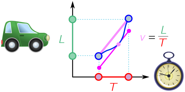
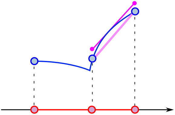
Finally, here’s a practical application: cheap traffic enforcement. Suppose traffic police monitor a stretch of highway of length $L$. They clock a car entering the stretch and leaving a time $T$ later. Without using a radar gun, they know from the MVT (see graph below) that the car was travelling at speed $v = L/T$ at some point along the stretch. If this is greater than the speed limit, they can issue a fine!

2.2. A kink in the argument

As fun as the MVT is to prove, it’s even more fun to break. If students draw a sharp kink in the curve, they will find that the theorem fails:

Although the blue curve lies entirely on one side of the purple line, the two never coincide, even when we zoom in. Put a different way, since the tangent to the blue curve isn’t even well defined, it cannot equal the purple line! This places an important technical constraint on the mean value theorem: at every point, the curve must be differentiable, aka straight at infinite zoom.

We could leave it there, but let’s try and maximally break the theorem. In the single-kink case, we can simply shift on the endpoints to define the function on a subinterval $a’ \leq x \leq b’$ where the mean value theorem does hold. We just avoid the kink!

So here is the challenge: define a continuous curve where the mean value theorem is not applicable in any subinterval. Since we can apply the theorem to any subinterval without kinks, we need every subinterval to contain a kink. In technical parlance, the kinks must be dense in $[a, b]$.

It’s hard to imagine (or draw) an infinitely jittery curve. But it’s easier if we proceed step-by-step. First, let’s set $a = 0$ and $b= 1$; we lose nothing by making this choice, since we can always scale and shift our answer to recover the result for an arbitrary interval. We can start with a trangle-shaped function possessing a single kink at $x = 1/2$. For the triangle, we can apply the MVT to any subinterval entirely to the left of the midpoint, or entirely the right of the midpoint. Call these intervals, where the MVT applies, good subintervals. They have maximum length $1/2$.

Our strategy will be to iteratively add more and more kinks, reducing the length of good subintervals by half each time until they disappear altogether! To begin with, let’s place kinks at $x = 1/4, 3/4$ so that the maximum length is $1/4$. A simple way to do this is to scale down the triangle function by a factor of 2, put two copies side by side, and add them to the big triangle, as depicted below. We label steps in the process by $n$, with $n = 0$ the big triangle with a single kink, and $n = 1$ the sum of big triangle and two smaller triangles.

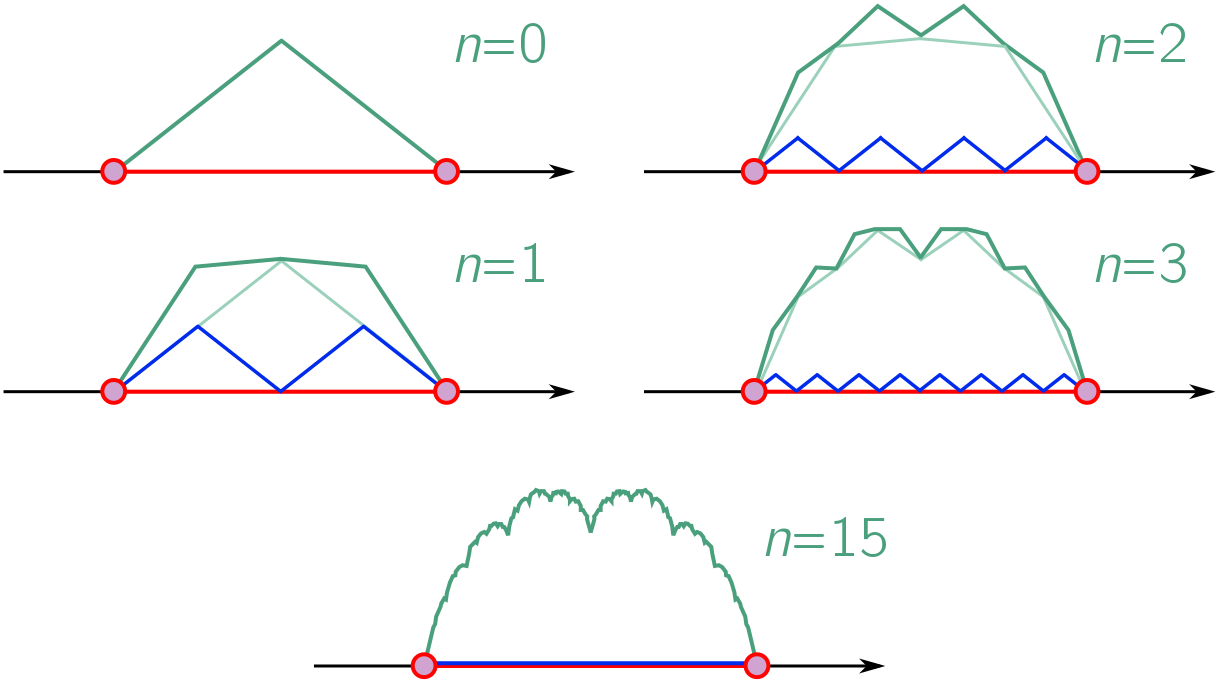
We can repeat this to obtain the $n = 2$ curve, shrinking the big triangle by a factor of $4 = 2^2$, making four copies, and adding to the $n = 1$ result. Now the maximum length of a good subinterval is $2^{-3} = 1/8$. Continuing in this fashion, at step $n$, we shrink the original triangle by a factor of $2^n$, spam $2^n$ copies, and add them to the results of the previous step. This iteratively builds up a fractal called the blancmange function, since it resembles the jellied mounds of the French dessert.

Good subintervals have maximum length $2^{-(1+n)}$. As $n$ gets larger and larger, this allowed length gets smaller and smaller, and in the limit $n \to \infty$, they have no length at all! Informally, this shows that for the blancmange function, there are no good subintervals. To make this slightly neater, we can label kinks with their “decimal” expansions in base 2. The initial kink is at $x = 0.1$. The kinks for $n = 1$ are at $x = 0.01, 0.10, 0.11$. The kinks for $n= 2$ are at

\[n = 0.001, 0.010, 0.011, 0.100, 0.101, 0.110, 0.111.\]

You get the idea: at stage $n$, there are kinks at all numbers $x\in (0, 1)$ with binary expansions of length $n+1$. In the limit $n \to \infty$, there will be a kink at every number $x \in (0,1)$ with a finite binary expansion. Like the finite decimal expansions we are used to working with, these binary expansions are indeed dense in the reals.

There are a few loose ends here. First, there is the question of pointwise convergence: is the blancmange function well-defined? If the students know the geometric series and the comparison test, they can prove this. A more delicate question is whether the function is continuous, requiring the M-test. In a classroom setting, I think it’s probably best to raise both problems, but answer them “experimentally”: simply graph the function at different values of $n$, or get the students to program it themselves. They should see the function settle down to something continuous as $n$ gets large. (See this Geogebra applet by David Richeson for example.) This is not a proof, but it does give a convincing numerical demonstration both of convergence and continuity.

Another question is why we bother adding the triangles. Why don’t we just take the limit of small triangles spammed together? This will have kinks at the same places as the blancmange.

It turns out that an infinitely small triangle is just a point, and $2^n$ small triangles make a line as $n\to\infty$. The technical tool to prove this is the Hausdorff limit of sets, but a simple intuition pump is simply to ask: how tall are the triangles as $n\to\infty$? If $f_n$ is the function consisting of $2^n$ triangles scaled down by $2^n$, what is the value of $f_n(x)$, for any $x$, as $n$ gets large? Everything just gets squished onto the red line.

To summarise, the blancmange function is continuous but nowhere differentiable, and a similar iterative construction for any single-kink curve gives a function with the same property. Some students will savour this pathological dessert, while others may not. They will be in good company. Towards the end of the 19th century, the mathematician Charles Hermite wrote, with typical fin de siècle bombast, “I turn with terror and horror from this lamentable scourge of functions with no derivatives”.

The moral is that, by trying to break theorems, ask bold questions, and follow loose threads, we often find something amazing lurking in the undergrowth. In their own way, monsters can be beautiful.

2.3. Slice of pi

I’ll do one more example, unrelated to the MVT, but returning to inverse trig derivatives. This requires a little more symbolic facility from students, but the payoff is a gorgeous (and useful) infinite series identity.

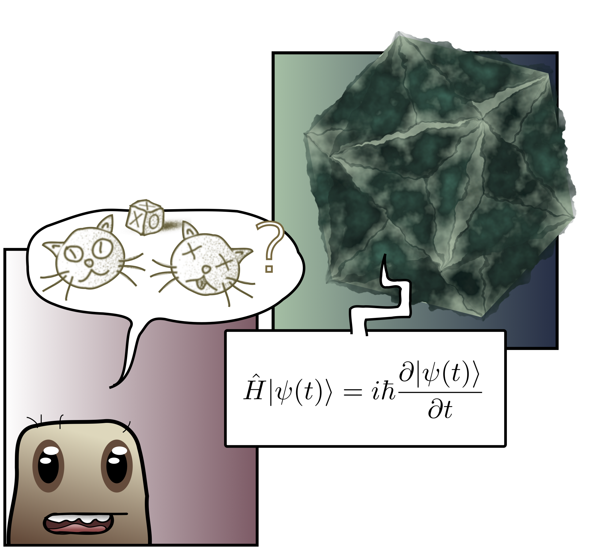
Infinite series deserve a greater place in the high school syllabus. When I first encountered them, I was astounded: they were beautiful but otherworldly, like a glittering chunk of meteorite found in the middle of a corn field. For instance, how could the formula

\[\frac{\pi^2}{6} = \frac{1}{1^2} + \frac{1}{2^2} + \frac{1}{3^2} + \frac{1}{4^2} + \cdots\]

possibly be true? And who could dream up a gewgaw like

\[\frac{1}{\pi} = \frac{2\sqrt{2}}{9801}\sum_{n=0}^\infty \frac{(4n)!(1103+26390n)}{(n!)^4 396^{4n}},\]

which Ramanujan seemed to do on a daily basis?

Although Ramanujan’s work still strikes me as semi-mystical, many results on infinite series, equally baffling and exciting to the outsider, are easy pickings with the long arm of calculus. In our case, we’ll cook up an infinite series for $\pi$ based on the inverse sine. First, recall the derivative:

\[\frac{d}{dx} \sin^{-1} x = \frac{1}{\sqrt{1-x^2}}.\]

The RHS can be expanded using the binomial series discovered by Isaac Newton:

\[(1-x^2)^{-1/2} = 1 + \frac{1}{2}x^2 + \frac{1\cdot 3}{2\cdot 4} x^4 + \cdots = \sum_{n-0}^\infty \frac{(2n)!}{2^{2n}(n!)^2} x^{2n}.\]

Is this too advanced for students? I don’t think so. It can be motivated as an extension of the usual binomial theorem, and “proved” (without worrying too much about convergence) via the Maclaurin series. Now “anti-differentiate” term-by-term:

\[\sin^{-1}x = x + \frac{1}{2}\frac{x^3}{3} + \frac{1\cdot 3}{2\cdot 4} \frac{x^5}{5} + \cdots = \sum_{n-0}^\infty \frac{(2n)!}{2^{2n}(n!)^2} \frac{x^{2n+1}}{2n+1}.\]

Here, the constant of integration is set to zero since inverse sine vanishes at $x = 0$. Finally, we plug in a specific value, $x = 1/2$:

\[\sin^{-1}(\tfrac{1}{2}) = \sum_{n-0}^\infty \frac{(2n)!}{2^{2n}(n!)^2} \frac{1}{2^{2n+1} (2n+1)}.\]

So what? Well, we know from “special triangles” that $\sin^{-1}(1/2) = \pi/6$. This yields the pleasing formula

\[\pi = 6\left[1 + \frac{1}{2}\left(\frac{1}{3\cdot 2^3}\right) + \frac{1\cdot 3}{2\cdot 4}\left(\frac{1}{5\cdot 2^5}\right) + \frac{1\cdot 3 \cdot 5}{2\cdot 4\cdot 6}\left(\frac{1}{7\cdot 2^7}\right) + \cdots\right].\]

As students can check themselves, this formula converges extremely rapidly. Below, I’ve plotted the first six partial sums.

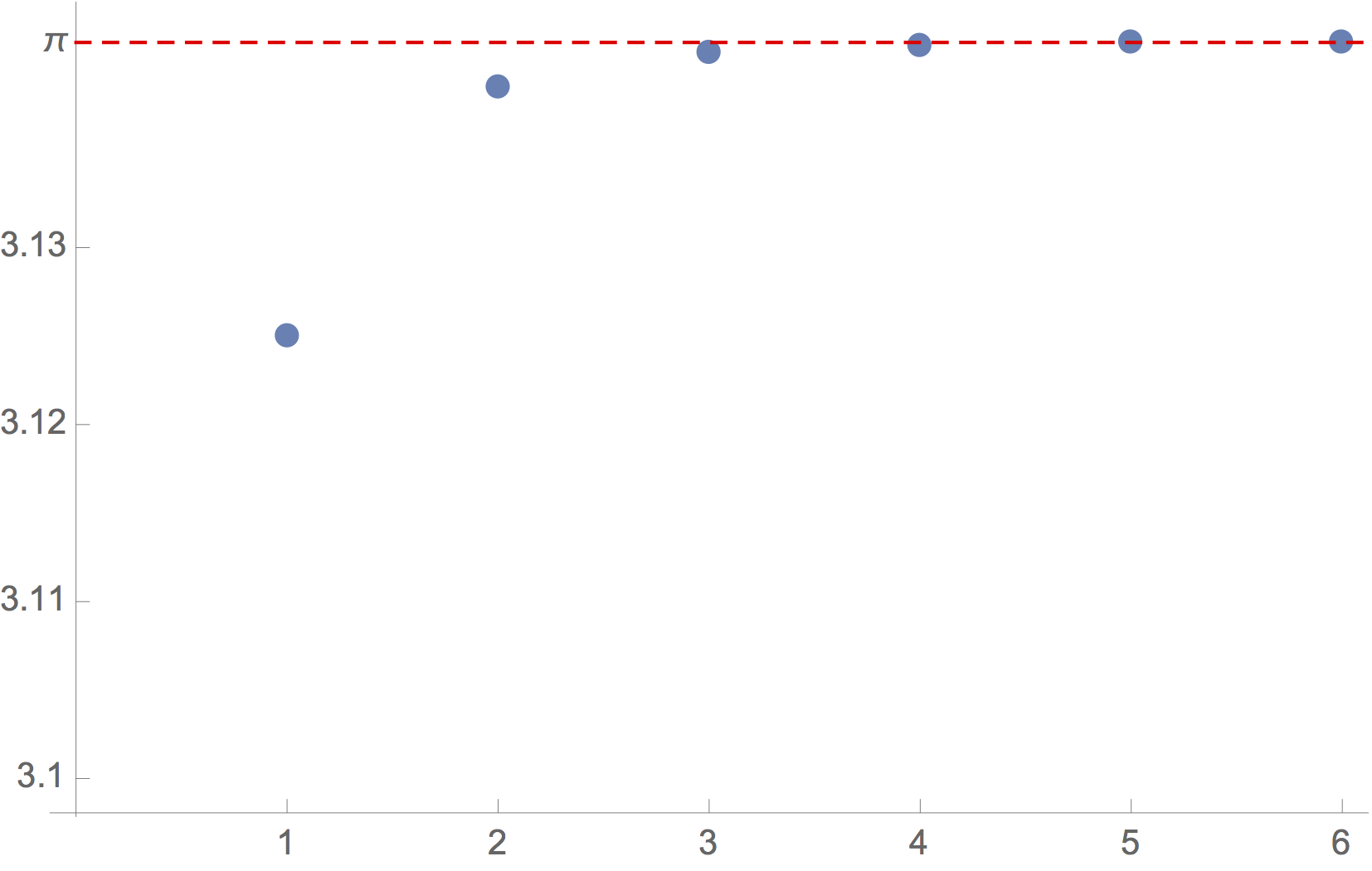
Newton himself derived this formula (using geometry rather than calculus) and exploited the rapid convergence to compute $\pi$ to $15$ decimal places in 1666. He later wrote, “I am ashamed to tell you to how many figures I carried these computations, having no other business at the time.” Students can reproduce this feat themselves! In fact, you can explore precisely how many terms are needed for a given number of digits.

For $15$ decimal places in $\pi$, you need only $19$ terms in the sum. More generally, the relationship between terms and decimal places is linear, as the graph above shows. You can get students to fit a line and predict how many terms they need for, say, the first $1000$ digits. They can add up terms and check that it’s right!

To derive Newton’s formula for $\pi$, we have thrown rigour to the wind. As with the blancmange, I think it’s worth mentioning the convergence issues at play (power series radius of convergence, uniform convergence for term-by-term differentiation) without belabouring them. On a first exposure, a quagmire of technical conditions will spoil the magic, and a numerical check can be just as convincing.

Is this pedagogically sound? I find the hiking analogy helpful here. Rigour is something like a heavy safety harness for mountain climbing. From the sheltered vantage of our hill, we can mention rigour and explain why the professional climbers need it, but do not ourselves need to gear up. There are other ways to orient students in the landscape and protect them from misadventure. That said, I see no reason that an advanced class should not try climbing a mountain every now and again, and prepare accordingly.

3. Mining for patterns

A second direction out of the scrubland is applied mathematics, understood broadly as the use of mathematics to solve problems in the real world. Unlike beauty, which never gets much of a rhetorical look in, the term “real world” is bandied about almost recklessly by maths teachers. In particular, the “real world” is the home (or perhaps graveyard) of word problems. Here are some examples from our textbook:

We have a shrinking moth ball, a growing triangle, and sand being poured into a conical pile. This is promising subject matter: objects in the real world which change with time. But nothing passes the shrub test! Why does the moth ball decrease at a constant rate? What causes the triangle to get bigger? Why is the conical angle of the sand pile precisely $71.57^\circ$? We’ve entered a surrealist fresco of melting objects labelled by irrelevant numbers.

Maths comes from the real world. In the same way that the material needs of civilisation spur on an explorer and frame her quest, the needs of science, industry, and everyday life spur mathematicians to go out into the landscape and dig up patterns fit for purpose. From compound interest to chaos, planetary motion to poker, and soap bubbles to ciphers, mathematics arises from real world needs. Why not let students in on the secret?

For maximum rhetorical impact, I’m going to redo the three word problems above. We will see that applied and pure maths are not mutually exclusive. When we dig up structures for real-world use, they often contain puzzles and extensions that lead to pure mathematical progress. This is a grand secret of mathematics: almost everything has pattern and structure on which mathematical tools can be brought to bear. (I hope to return to this theme at length in the future.)

3.1. Sublime moth balls

We start with moth balls, adapting and simplifying the lovely article by Tennakone and Pieris (1978). We’ll see how the size of spherical moth balls really changes with time. Students can use this information to experimentally determine microscopic properties of air, just by waiting for a moth ball to decay!

Moth balls are made out of a chemical called napthalene ($\text{C}_{10}\text{H}_8$). A sphere of napthalene will shrink as the molecules on the surface layer sublime, i.e. turn directly from solid to gas. Assuming the rate of sublimation is uniform over the surface, the moth ball remains approximately spherical.

The sublimed napthalene forms a spherical cloud of gas around the moth ball, spreading outward or diffusing due to the random motion of the molecules. Let $c(r)$ be the concentration of gas (number of molecules per unit volume) around the ball, defined as a function of radial distance $r$ from the ball’s centre. For a very thin spherical shell of width $w$ (where $c(r)$ is effectively constant over the shell), the rate at which molecules diffuse out of the shell is proportional to the concentration $c(r)$ and velocity $v$ of molecules.

---

1. Consider two thin shells, one at radius $r$ and another at radius $r + w$. Assuming the velocity of molecules is fixed for all shells, explain why the net rate $F$ of molecules leaving the second shell (at radius $r+w$), per unit area, is proportional to

   \[F(r+w) \propto \frac{c(r+w)-c(r)}{w}.\]

2. By taking the limit of zero width, show that the net outward flow of molecules from the shell at radius $r$, per unit area, is

   \[F(r) = D \frac{dc(r)}{dr},\]

   where $D>0$ is a constant of proportionality called the diffusion constant.

3. Suppose the napthalene cloud diffuses very slowly, with a steady outward flow of molecules. Argue that, for this steady flow, the function

   \[G(r) = 4\pi r^2 F(r)\]

   must be constant.

4. Let $R$ be the radius of the moth ball. From Problem 3, deduce that

   \[c(r) = \frac{c(R) R}{r}.\]

   Since the rate of sublimation is uniform, the concentration $c(R)= c_\text{sub}$ at the surface of the moth ball is independent of $R$.

5. Since the moth ball is gradually turning into gas, the radius $R(t)$ depends on time. It is a little easier to calculate how the mass of the ball changes with time. Show that if $m_\text{N}$ is the mass of a napthalene molecule, and $M$ the mass of the moth ball, then

   \[\frac{dM}{dt} = -m_\text{N}G(R) = -4 \pi m_\text{N} c_\text{sub}D R.\]

6. If $\rho$ is the mass density of the moth ball, show that we can rewrite the rate of change of mass in Problem 5 as a rate of change of radius:

   \[\frac{dR}{dt} = -\frac{D c_\text{sub} m_\text{N}}{\rho R}.\]

7. By explicit differentiation, check that the equation in Problem 6 is solved by

   \[R(t) = \sqrt{R_0^2 - \left(\frac{2D c_\text{sub} m_\text{N}}{\rho}\right) t},\]

   where $R_0$ is the radius at time $0$. Infer that the lifetime of the moth ball is

   \[t_\text{life} = \frac{\rho R_0^2}{2D c_\text{sub} m_\text{N}}.\]

8. (Experiment) A single molecule of napthalene weighs around $m_\text{N} = 2.1 \times 10^{-22} \text{ g}$. At room temperature, the surface concentration of napthalene is $c_\text{sub} = 3.3 \times 10^{22} \text{ m}^{-3}$. Buy some moth balls, and measure their initial radius $R_0$ and density $\rho$. Leave them in a cool dry place and see how long they take to disappear, i.e. determine $t_\text{life}$. From Problem 7, estimate the diffusion constant for napthalene in air.

---

3.2. Irodov’s triangle

Our next problem extends the classic pursuit puzzle first posed in Igor Irodov’s Problems in General Physics and later popularised by Martin Gardner. Three homing missiles $M_1, M_2, M_3$ are fired at each other from the vertices of an equilateral triangle. The triangle has side $\ell$, and missile $M_1$ homes in on $M_2$, $M_2$ on $M_3$, and $M_3$ on $M_1$.

Assume the missiles have the same speed profile over time, $v_1(t)=v_2(t)=v_3(t)=v(t)$. The danger zone is the triangle formed by three missiles. This is where you might get hit!

Part I: Meeting in the middle

---

1. Argue that the danger zone (pictured above) is always an equilateral triangle.

2. Using Problem 1, explain why the missiles always point in directions separated by angle $\theta = 2\pi/3$.

3. From Problem 2, show that the relative speed at which $M_1$ and $M_2$ approach each other is

   \[v_{12}(t) = [1 - \cos\theta]v(t).\]

4. How far does each missile travel before colliding at the centre? (No calculus needed.)

5. Extending your observation in Problem 4, explain why the paths traced by the missiles do not depend on their velocity, provided the speed profiles agree.

6. (Extension) Generalise your result to $n$ homing missiles on the vertices of an equilateral polygon, with $n$ sides of length $\ell$. What happens in the limit as $n\to\infty$, if we shrink the sides as $\ell/n$? Does you answer make sense?

---

The fact that the danger zone remains equilateral tells us a beautiful fact about the path of the missiles: it is self-similar, in the sense that as we zoom in, the shape is the same. Set up polar coordinates $(r, \phi)$ with the origin at the centre of the danger zone. A path $r = f(\phi)$ in polar coordinates is self-similar if zooming in (multipling $r$ by a constant) only shifts the angle:

\[\begin{equation} \alpha r = f(\phi - c),\label{self} \tag{1} \end{equation}\]

where $c = c(\alpha)$ depends on $\alpha$. This allows us to actually work out the curves!

Part II: Self-similar spirals

---

1. Differentiate both sides of (\ref{self}) with respect to $\alpha$, and set $\alpha = 0$, to find that

   \[f(\phi) = -f'(\phi) c'(0).\]

2. Verify directly (or solve a separable DE to show) that this equation is solved by

   \[f(\phi) = C e^{-c'(0)\phi}\]

   for some constant $C$. Thus, any self-similar curve in polar coordinates takes the form of a logarithmic spiral,

   \[r = C e^{-k\phi},\]

   for constants $C$ and $k$.

3. Choose coordinates so that the missiles initially lie at angles $\phi = 0, 2\pi/3, 4\pi/3$. Show that the curve associated to the first missile (at $\phi = 0$) is a logarithmic spiral with $C = \ell/\sqrt{3}$ and $k = \sqrt{3}$. The remaining two curves are simply rotated by $\pm 2\pi/3$ around the origin.

   Hint. The derivative $r’(\phi)$ at $\phi = 0$ tells us the direction the missile points.

4. (Extension) Determine the spirals for a polygon of $n$ homing missiles.

---

This problem is beautiful because symmetry (rotational and scaling) solves the problem for us. We still need derivatives, but they now have the nontrivial role of extracting the logarithmic spiral from self-similarity, and determining parameters for the path of the missiles. Swiss mathematician Jacob Bernoulli called this curve the spira mirabilis (“marvellous spiral”) since he was so struck by its property of self-resemblance. His gravestone even bears the enigmatic Latin phrase

Eadem mutato resurgo. (Although changed, I shall arise the same.)

This apparently refers to the self-similar spiral.

3.3. Sand piles, slopes and self-organisation

Our final revision is the sand pile, taking inspiration from the model of Bouchard, Cates, Prakesh and Edwards (1994). They split a pile of sand into two components: a standing layer, which is the large blob of stable sand at the bottom of the pile, and a rolling layer of loose grains running down the slope.

The height of the standing layer is denoted $S$, and the thickness of the rolling layer on top is called $R$. The total height of the sand pile is then

\[H = S + R.\]

The angle of repose $\theta_\text{rep}$ is the maximum angle of a stable sand pile; for simplicity we use the slope $\alpha = \tan\theta_\text{rep}$. If a patch on the standing layer has slope greater than $\alpha$, it will shed grains into the rolling layer. If it has slope less than $\alpha$, a rolling layer can deposit grains onto the pile.

To make life easy, we just deal with one-dimensional piles. Zoom in on a patch of sand pile centred at $x$, width $w$, small enough that both the standing and rolling layer have constant slope, $m$ and $\kappa$ respectively.

Let’s first see how the height of the standing layer changes with time. A reasonable guess is that sand grains move between the layers at a rate proportional to (a) the current thickness $R$ of the rolling layer, and (b) the difference between the standing slope and the angle of repose. This means we can write the rate of change of $S$ as

\[\begin{equation} \frac{dS}{dt} = \gamma r(\alpha - m), \label{ds/dt} \tag{2} \end{equation}\]

for some constant of proportionality $\gamma$ depending on the properties of the sand. Note that the value of $R$ here is evaluated in the middle of the patch at $x$, as is the value of $S$. Now we turn to the rolling layer, and use our equations to solve for the shape of a simple triangular sand pile.

---

1. Assume the density of sand is the same in the standing and rolling layer. Explain physically why a change in $S$ doesn’t affect the total height $H$.

2. Let $\kappa$ be the slope of the rolling layer, defined as in the picture. In a short time $\Delta t$ (short enough that $\kappa$ remains approximately constant), show that the area of rolling sand above our patch changes by $\Delta A = -vw\kappa\Delta t$.

3. Given the result of Problem 1, the only way to change $H$ is for the size of the rolling layer to change. Show that $H$ is related to the total area of sand above the patch by $A = Hw$.

4. Using Problems 2 and 3, argue that the total height of the sand pile at $x$ changes according to

   \[\frac{dH}{dt} = -v\kappa.\]

5. Suppose we begin pouring sand from a bucket into the patch at some rate $bw$. If this sand starts rolling immediately, show that the change in height becomes

   \[\begin{equation} \frac{dH}{dt} = -v\kappa + b. \label{dh/dt} \tag{3} \end{equation}\]

   Conclude that the rolling layer of the patch thins out at rate

   \[\frac{dR}{dt} = -v\kappa + b-\gamma R(\alpha - m).\]

6. (Extension) Consider a triangular pile of sand on a base of width $B$, with a steep drop on either side so the rolling layer falls off rather than building up. Suppose the standing layer is at the angle of repose. We focus on the right side of the triangle by symmetry.

   (a) Show that when $b = 0$, the sand pile equations imply

   \[R(x, t) = R(x - vt).\]

   This dependence on $x-vt$ is the mathematical definition of a wave.

   (b) A child now pours a thin, time-dependent stream of sand onto the top of the pile. This sets the height of the rolling layer at the top of the pile for each time $t$:

   \[R(0, t) = C(t).\]

   Assuming $b = 0$ for $x > 0$, show that the profile of the sand pile for $B/2 \geq x \geq 0$ is

   \[\begin{equation} H(x, t) = \frac{1}{2}\alpha B - \alpha x+ C(t-x/v).\label{tailings1} \tag{4} \end{equation}\]

---

The BCPE sand pile model shows how slopes in time and space interact, and leads to the insight that the rolling layer travels like a wave down a standing cone at the angle of repose. I think this is rather nice, and clearly beyond the scrubland. But there’s a spectacular twist to the story of sand piles if we consider discrete models. I won’t delve into the details, though I think they could form the basis of a meaty programming project for a keen class.

Imagine dropping sand grains at random onto a discrete grid of points. If too many grains build up at a single site, they spill onto neighbouring sites. If any of these neighbouring sites are full, they too can spill, with the result that a single grain can cause an avalanche which redistributes some large portion of grains in the sand pile. This is, in brief, the Abelian sand pile of Bak, Tang and Weisenfeld (1987). It has many remarkable properties, such as a pretty fractal structure in the distribution of grains when run for long enough:

This fractal is related to the deeper property of self-organised criticality, where the sandpile “tunes” itself to maintain a delicate balance between total order (no avalanches) and disorder (too many avalanches). The technical tool to assess this balance is the statistical relation between size and frequency of avalanches. I won’t discuss it here, but this is something students can easily see for themselves in computer simulations.

According to Steven Krantz, there is an infamous MIT exam which simply reads:

You have a pile of warm metal shavings in the shape of a cone. Discuss.

I can think of worse topics than this extraordinary connection between piles of granular matter and self-organising fractals.

4. Miscellaneous issues

In this final section, I want to address a few pitfalls and sketch some ideas about classroom implementation.

How do students develop basic skills?

As mentioned earlier, drill is much more bearable when there are real applications on the horizon. But I suspect the act of drilling itself can be made more palatable with a little effort. Consider these two examples:

---

1. Differentiate the following and state the maximal domain:

   (a) $\sin^{-1}(x/3)\qquad$ (b) $\cos^{-1}(x^2)\qquad$ (c) $\tan^{-1}(\sqrt{x})$.

2. (a) Using the chain rule, find the derivative of $f(x) = \cos(\sin^{-1}(x))$.

   (b) Deduce from trigonometric identities that $f(x) = \sqrt{1-x^2}$. Do the domains match? Differentiate and check that your answer agrees with (a).

   (c) Implicitly differentiate $\cos^{-1} y = \sin^{-1} x$ and isolate the expression for $dy/dx$. Is this consistent with your previous answers?

---

Which is better? I would argue that the second passes the shrub test while the first does not, though they develop the same skills: differentiating inverse trigonometric functions, using the chain rule, and identifying domains.

There is much more to say about how we teach basic skills. I think a constructivist approach which breaks material into small, bite-sized pieces (see JUMP math for an example at the primary level), and which takes different learning styles into account (employing heuristics, visual aids, computers, and colourful analogies) could dramatically improve engagement and retention. But my focus here has been on how to leave the scrubland, rather than the best way to develop walking skills. I intend to return to this in a later post!

Does this work for pre-calculus topics?

Of course! I literally chose calculus at random from the textbook. Any mathematical topic has gorgeous theorems, freakish specimens, and a rich history of real-world motivation and use. Teaching trigonometry? Perhaps Euclid is a little dry, but what about non-Euclidean geometry? This is a wonderful place for guided discovery and exploration. (Robert and Ellen Kaplan, on the other hand, have designed some Math Circle courses around the special properties of triangles. See their inspiring book Out of the Labyrinth.) And what could be more empowering than determining the size of the earth from the shadow of a stick, as Eratosthenes did in 100 BC? For algebra, try the unsolvability of the quintic, compass and straightedge constructions, and applications to dimensional analysis. Logarithms? Here we have the density of prime numbers, slide rules, algorithmic complexity and Fermi estimates. The list goes on.

Hopefully the idea is clear. Pick a topic, any topic. Figure out its history, where it comes from, what it’s really used for and what mathematicians or scientists find beautiful about it. Now incorporate that material into the syllabus. Mathematical skills live in a big constructivist framework, and according to the maximin test, attention needs to be paid to developing that framework so that all students can benefit. But if we can productively interleave the two, with basic skills giving access to highlights, and highlights motivating the practice of new skills, these goals are not at odds!

What is the teacher’s role?

In the approach I’m suggesting, the role of the teacher seems to be supplanted by a curriculum full of sparkling ideas. But learning is a relational endeavour, and the teacher remains an essential part — probably the essential part — of the process. It is through the teacher that trust is established, students are engaged, and the subject comes alive. They also provide careful guidance and feedback during the process of learning to walk.

For all of this to happen, teachers need to be on top of the material. If the syllabus now encompasses continuous but nowhere differentiable functions, numerical approximation, diffusion, and self-organised criticality, it seems like an impossible ask for all but the most specialised of high school maths teachers. But here’s the trick: if students can learn it, so can teachers! Once they’ve left the scrubland, teachers can stop trotting out the same dubious cliches about using maths in real life, and get genuinely excited about what they teach. Their enthusiasm will be infectious.

Why are the problems in section 3 so hard?

This post is partly an experiment with format. The first experiment was informal, expository and visual (section 2), while the second experiment was an attempt to turn difficult problems into bite-sized chunks (in section 3). I’m not sure the latter succeeded, but the point of the experiment is to try!

What’s next?

Instead of replacing the curriculum (an overambitious goal), paths out of the scrubland can be offered as a complement to standard material. In the near future, I hope to start assembling a database of extensions, theorems and applications, embedded in a constructivist framework and cross-referenced against real curricula. Watch this space!

5. Conclusion

Teachers and curriculum writers are experts on modelling what students know and how they come to know it. Scientists and mathematicians are domain experts, with specialised knowledge, taste, and judgment. By working together, they can decide how to lead students out of the scrubland, and into the vast topography of the real mathematical world, with its majestic summits, calm valleys and extraordinary wildlife. From its fertile soil, students can grow new plants and mine for patterns, fit for the as-yet-unknown mathematical needs of the 21st century. And even more importantly, they can enjoy the simple pleasures of mathematics, which have for so long, and so unnecessarily, been denied to most students.

Annotated bibliography

Here are some books and articles I found useful or inspiring while writing this post. I’ve included some brief annotations.

• “Self-organised criticality: an explanation of 1/f noise” (1987), Per Bak, Chao Tang and Kurt Weisenfeld. An explosive paper which started a new field of study. Unfortunately, real sand piles don’t seem to behave this way, but the model remains provocative and useful.
• “A model for the dynamics of sandpile surfaces” (1994), J.-P. Bouchard, M. E. Cates, J. Ravi Prakesh and S. F. Edwards. A simple model of sand piles, fleshing out the insights of Nobel-prize winner Pierre-Gilles de Gennes.
• “Darwin’s Tree of Nature and other images of wide scope” (1981), Howard Gruber. In Aesthetics in Science, ed. Judith Weschler. A beautiful essay about scientific imagery, intuition, and the aesthetics of complexity. I think the fascination of the blancmange and other “pathological” examples holds the same appeal as the tangle of roots on a riverbank did for Darwin.
• A Mathematician’s Apology (1940), G. H. Hardy. The classic apologia for pure mathematics. Hardy somewhat amusingly insists on the uselessness of special relativity (atomic energy) and number theory (cryptography), which I think goes to show that use and beauty will always be intertwined.
• Problems in General Physics (1981), Igor Irodov. A concise, Soviet-style introduction to mechanics, with a great array of problems.
• Out of the Labyrinth (2007), Ellen and Robert Kaplan. An inspiring manifesto on the Kaplans’ method for teaching mathematics via play and exploration in the Harvard Maths Circle. It is even more radical than the approach I am suggesting here!
• The Myth of Ability (2003), John Mighton. An exposition of the JUMP method, a constructivist framework for teaching everyone how to walk. The data from the JUMP method shows that a maximin ethic really does benefit everyone.
• “Reinventing explanation” (2014), Michael Nielsen. An inspiring and comprehensive look at new ways to explain science using “cognitive media”. (See also Bret Victor.)
• “Sublimation of moth balls” (1978), M. G. C. Peiris and K. Tennakone. A cute AJP article on moth ball sublimation.
• A Theory of Justice (1971), John Rawls. The most influential book on political philosophy and liberalism of the 20th century.
• “The Mathematical Unconscious” (1981), Seymour Papert. In Aesthetics in Science, ed. Judith Weschler. A perceptive essay on aesthetics and mathematical intuition from one of the giants of old-school AI.
• “Up and down the ladder of abstraction” (2011), Bret Victor. A brilliant essay on the use of interactive (or cognitive) media to facilitate abstraction. I disagree with Victor’s claim that only a select few have the “freakish knack” for manipulating symbols, but agree with Victor and Nielsen that cognitive media can and should complement traditional symbolic methods.
• “Abstraction, intuition, and the monad tutorial fallacy” (2009), Brent Yorgey. Analogies are great, but not a silver bullet. Yorgey argues that intuition-building and play should precede analogy-making.