November 28, 2020. I discuss some of the key properties of the exponential function without (explicitly) invoking calculus. Starting with its relation to compound interest, we learn about its series expansion, Stirling’s approximation, Euler’s formula, the Basel problem, and the sum of all positive numbers, among other fun facts.

Contents

1. Compound interest
2. An infinite polynomial
3. From interest to small change
4. Stirling’s approximation
5. Euler’s formula
6. Factorization and the Basel problem
7. Ramanujan’s mysterious sum*

1. Compound interest

Suppose you make an investment $I_0$ which promises a return rate $r$ per year. The simplest possibility is that, at the end of the year, you generate some interest $r I_0$, so the total value of the investment is $I_\text{simp} = (1+r)I_0$. This is called simple interest. But what if, instead, you get paid in six month instalments? At the end of the first six months, you should get paid half your interest, or $I_0 (r/2)$, so the total value is

\[I_1 = \left(1 + \frac{r}{2}\right) I_0.\]

If the interest is simple, you get the same amount of interest $(r/2)I_0$ at the end of the year. But if instead of simple interest you have compound interest, then the interest for the second half of the year is recalculated based on its value after six months. In other words, the second interest payment will be $(r/2) I_1$ rather than $(r/2) I_0$, leading to a total value

\[I_{\text{comp}(2)} = \left(1 + \frac{r}{2}\right) I_1 = \left(1 + \frac{r}{2}\right)^2 I_0.\]

For a positive interest rate, $I_1 > I_0$, so you will get more interest in the compound scheme. Mathematically, $I_{\text{comp}(2)} > I_\text{simp}$ because

\[\left(1 + \frac{r}{2}\right)^2 = 1 + r + \frac{r^2}{4} > 1 + r.\]

Of course, I chose six months arbitrarily. I could split the year into $n$ equal lengths, and use those to compound interest, i.e. recalculate the next instalment based on the current value, including the interest generated so far. Let’s call this value $I_{\text{comp}(n)}$. As $n$ increases, so will the total value $I_{\text{comp}(n)}$ of our investment, and in fact it has the value

\[I_{\text{comp}(n)} = \left(1 + \frac{r}{n}\right)^n I_0\]

since the interest rate for any period is $r/n$, so we multiply by $1 + r/n$ at the end of each period. A natural question is: how big can the interest at the end of the year get? Will it get infinitely large as I make $n$ large, or will it approach some finite value? Mathematically, this is just the question:

\[\lim_{n\to \infty}\left(1 + \frac{r}{n}\right)^n = \,\,?\]

It turns out this has a finite limit! Proving this is actually rather difficult, but it’s easy to see with a computer. We can just plot $(1+r/n)^n$ for increasingly large $n$ and see that it settles to a finite value.

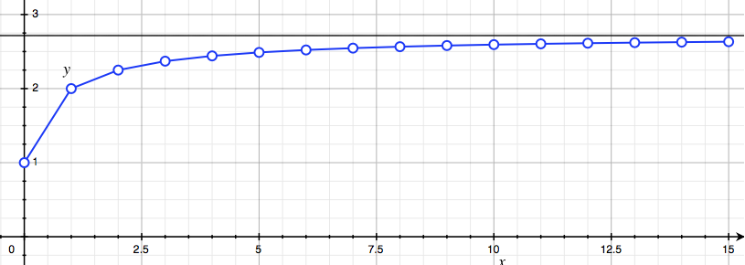
We show a few values for $r = 1$ above. For large $n$, say a million, we get a number $2.71828…$, plotted as the horizontal black line. Assuming it does converge, we use the $r =1$ limit to define the famous mathematical constant $e$:

\[e = \lim_{n\to\infty} \left(1 + \frac{1}{n}\right)^n \approx 2.781828.\]

We’ll return to the mathematical question of convergence below.

---

Exercise 1. Show that in the limit of “continuous” compound interest, i.e. large $n$, the total value of our principal $I_0$ at the end of the year is

\[\lim_{n\to\infty} I_{\text{comp}(n)} = e^r I_0.\]

You can assume that

\[\lim_{n\to\infty} x_n^r = \left[\lim_{n\to\infty} x_n\right]^2.\]

Hint. Consider redefining $n$ so that the interest term looks more like the definition of $e$.

---

Assuming this limit of continuous compounding exists, we define the exponential function as

\[e^x = \lim_{n\to\infty} p_n(x), \quad p_n(x) = \left(1 + \frac{x}{n}\right)^n,\]

where for convenience, we’ve defined the polynomial $p_n(x) = (1+x/n)^n$. Thus, if the interest rate per annum is $r$, and we compound with $n$ intervals, the total value at the end of the year is $p_n(r)I_0$. In the rest of this post, we will explore some of the remarkable properties and applications of the exponential function, but from an elementary, pre-calculus point of view.

2. An infinite polynomial

Above, we expanded the term $p_2(x)$:

\[p_2(x) = \left(1 + \frac{x}{2}\right)^2 = 1 + x + \frac{x^2}{4}.\]

With a bit more labour, we can expand out the expression for three periods, $p_3(x)$:

\[p_3(x) = \left(1 + \frac{x}{3}\right)^3 = 1 + x + \frac{x^2}{3} + \frac{x^3}{27}.\]

These are different polynomials, but the first two terms are the same. More generally, we can ask: what do the polynomials $p_n(x) = (1+x/n)^n$ look like? And like the $1$ multiplying $x$, do coefficients in the polynomial $p_n(x)$ “stabilize” as $n$ gets large? Our tool to explore this will be the binomial theorem. This states that

\[(1 + X)^n = 1 + \binom{n}{1}X + \binom{n}{2}X^2 + \cdots + \binom{n}{n}X^n,\]

where

\[\binom{n}{k} = \frac{n!}{(n-k)! k!}\]

is the number of ways of choosing $k$ from $n$ objects, also called a binomial coefficient. I’m going to assume you know about binomial coefficients, but not necessarily the binomial theorem. But if you know about binomial coefficients, the theorem is easy!

When we expand $(1+X)^n$, we can generate terms by choosing either $1$ or $X$ in each factor. To obtain a term $X^k$, in $k$ factors we choose $X$, and in the remaining factors we choose $1$. We add all our choices together to get the final answer, so the total number of ways to get $X^k$ (and hence the coefficient) is just the number of ways we can choose $k$ from a total of $n$ factors, $\binom{n}{k}$. Done! Now we can figure out what the coefficient of $x^k$ looks like in $p_n(x)$. Setting $X = x/n$ in the binomial theorem, we find that

\[p_n(x) = \left(1 + \frac{x}{n}\right)^n = 1 + \binom{n}{1}\frac{x}{n} + \binom{n}{2}\frac{x^2}{n^2} + \cdots + \binom{n}{n}\frac{x^n}{n^n}.\]

For $k \leq n$, the coefficient of $x^k$ is

\[\binom{n}{k}\frac{x^k}{n^k} = \left[\frac{n!}{(n-k)! n^k}\right] \frac{x^k}{k!},\]

where we’ve separated it into a part which depends on $n$ and a part which doesn’t. Let’s focus on the stuff which depends on $n$, and see if we can understand what happens when $n$ gets large. We can write

\[\begin{align*} \frac{n!}{(n-k)! n^k} & = \frac{n \times (n-1) \times \cdots \times (n-k+ 1)}{n^k} \\ & = \left(\frac{n}{n}\right) \times \left(\frac{n-1}{n}\right) \times \cdots \times \left(\frac{n-k + 1}{n}\right), \end{align*}\]

where we’ve paired the factors of $n$ downstairs with factors of $n!/(n-k)!$ upstairs. If we fix $k$, and let $n$ get very large, each of these terms gets very close to $1$. For instance, each term is bigger than

\[\frac{n-k}{n} = 1 - \frac{k}{n},\]

and as $n \to \infty$ with $k$ a fixed number, this approaches $1$. So each term approaches $1$, and hence the product approaches $1$ as $n$ gets large. So we conclude that, as we take $n \to \infty$, the coefficient of $x^k$ in $p_n(x)$ approaches $1/k!$. We can view the exponential function as $p_\infty(x)$, a sort of infinitely large polynomial with these coefficients:

\[e^x = p_\infty(x) = 1 + x + \frac{x^2}{2!} + \cdots + \frac{x^k}{k!} + \cdots.\]

This can be rigorously established, and the infinite polynomial $p_\infty(x)$ is called a power series. But we will continue to play fast and loose with the rules, ignoring the messy (and distracting) business of formal proof.

---

Exercise 2. The numerical approximation to $e$ from evaluating $p_n(1)$ is very slow. We present a much quicker algorithm here.

(a) Express $e$ in terms of the power series $p_\infty(x)$.

(b) From your answer to (a), create a method for approximating $e$ using $k$ rather than $n$. Use this to estimate $e$ to $10$ decimal places. How many terms do you need?

---

3. From interest to small change

Another unique property of the exponential is how it responds to small changes. Consider some tiny $\delta \ll 1$. The usual index laws and the power series tell us that

\[e^{x + \delta} = e^x e^{\delta} = e^x \left(1 + \delta + \frac{\delta^2}{2!} + \cdots\right).\]

If $\delta$ is very small, then most of the change is captured by the linear term in the polynomial, $e^\delta \approx 1 + \delta$, since all the higher terms, proportional to $\delta^2, \delta^3$, and so on, are miniscule. More precisely, taking $\delta \ll 1$ and multiplying both sides by $\delta$, we find that $\delta^2 \ll \delta$, and hence $\delta^3 \ll \delta^2 \ll \delta$, and so on. For instance, if $\delta = 0.001$, then

\[e^\delta = 1.00100050\ldots \approx 1.001 = 1 + \delta.\]

Our linear approximation has an error of less than one part in a million. Thus, under a very small change $\delta$,

\[e^{x+\delta} - e^x \approx e^x \left[(1 + \delta) - 1\right] = \delta e^x.\]

So the response to a small change is proportional to the function itself. This actually gives another way to define the exponential! But more importantly, it underlies the many application of the exponential to real-world phenomena.

---

Exercise 3. A sample of Uranium-235 awaits testing. It has a half-life of $\lambda = 700$ million years, meaning that if there is a lump of $N$ Uranium-235 atoms, half of it will disappear after a time $\lambda$.

(a) Suppose we start with $N_0$ atoms. Using the analogy to compound interest, argue that the number of atoms after time $t$ is (to a good approximation)

\[N(t) = N_0 e^{-t/\lambda}.\]

(b) If there are $10^{26}$ atoms in a lump, roughly how long does it take for a single atom to decay? Hint. Use the formula for small changes.

---

4. Stirling’s approximation

We have just seen an approximation that works for very small arguments of the exponential. In this section, we present a rough guess for large arguments, which leads in turn to a beautiful approximation of the factorial. This is called Stirling’s approximation after James Stirling, though credit should also go to Abraham de Moivre who discovered it slightly earlier. The basic idea is to consider $e^n$. From our infinite polynomial, this can be written

\[e^n = 1 + n + \frac{n^2}{2!} + \cdots + \frac{n^k}{k!} + \cdots.\]

If we start counting from $k = 0$, the $k$th term is

\[a_k := \frac{n^k}{k!} = \left(\frac{n}{1}\right) \times \left(\frac{n}{2}\right) \times \cdots \times \left(\frac{n}{k}\right).\]

This gets progressively larger while $n \geq k$. But once we hit $n = k$, the subsequent factors will be less than $1$, so it begins to shrink again. The nearby terms are of similar size, but soon they begin to shrink and become negligible. We plot the terms $a_k$ for $n = 10$, from $k = 0$ to $k = 20$ below:

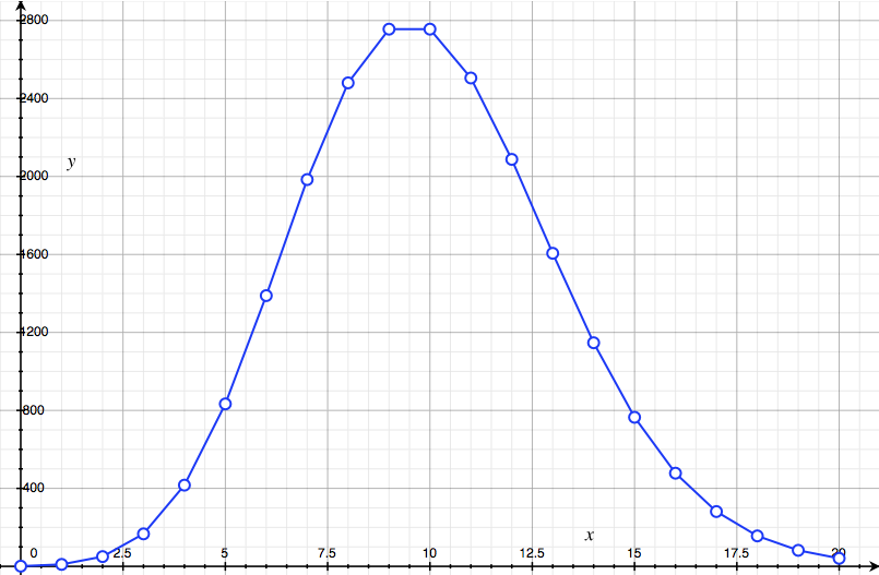
It starts small, peaks at $k = 9, 10$, then quickly drops down again. Our guess is very simple: the total value $e^n$ is proportional to this maximum value,

\[e^n = C_n a_n = C_n \frac{n^n}{n!},\]

with some constant of proportionality $C_n$ to account for the contribution of other terms. From the picture, it seems plausible that $e^n$ (which comes from adding all the dots) is much smaller than $n$ dots of height $a_n$, and hence

\[e^n = C_n a_n \leq n a_n \quad \Longrightarrow \quad C_n \leq n.\]

This is a very sloppy estimate of $e^n$ because of the factor of $C_n$. But we can turn this into a good estimate of something else, simply by taking logarithms. I assume you know about logs, and in particular, that taking log to the base $e$ makes sense, but as a quick reminder, here is the defining equation:

\[\log_e x = y \quad \Leftrightarrow \quad e^y = x.\]

We write $\log_e$ as $\ln$ for “logarithm natural”, as the French would have it. If we take logs of $e^n = C_n a_n$, the LHS gives

\[\begin{align} \ln e^n & = n \ln e = n, \end{align}\]

while the RHS gives

\[\ln (C_n a_n) = \ln C_n + \ln n^n - \ln n! = \ln C_n + n\ln n - \ln n!.\]

Since $C_n \leq n$, $\ln C_n$ is much smaller than the other terms in the equation, so we can throw it away! Combining the two equations and rearranging a little gives Stirling’s approximation:

\[\ln n! \approx n\ln n - n.\]

As a quick example, we can estimate

\[\ln 100! \approx 100 \ln 100 - 100 \approx 361.\]

Evaluating $\ln 100!$ exactly on a calculator gives $364$, an error of less than $1$%!

---

Exercise 4. Unfortunately, proving that $C_n \leq n$ takes a bit more time and machinery than we can afford. Rather than mend our sloppy ways, we will dig in, and estimate $C_n$ using guesswork and computers! Our first inspired guess is that the curve we plotted for $n = 10$ looks like a Bell curve! This is a ubiquitous probability distribution that traits like height and weight obey. A Bell curve with mean $\mu$ and standard deviation $\sigma$ has two important properties:

• It has a maximum height of $1/\sigma\sqrt{2\pi}$ at $\mu$.
• A distance $\sigma$ to the left or right of $\mu$, the probability drops to around $0.6$ of its maximum height.

Over to you!

(a) The area under the curve made by the points $a_k$ is around $e^n$, since we add them all up to get this value. Argue that, if the $a_k$ do describe an approximate Bell curve, it must be scaled vertically by a factor $e^n$, and hence has a maximum height

\[h = \frac{e^n}{\sigma\sqrt{2\pi}}.\]

(b) Assuming (a) is true, deduce that

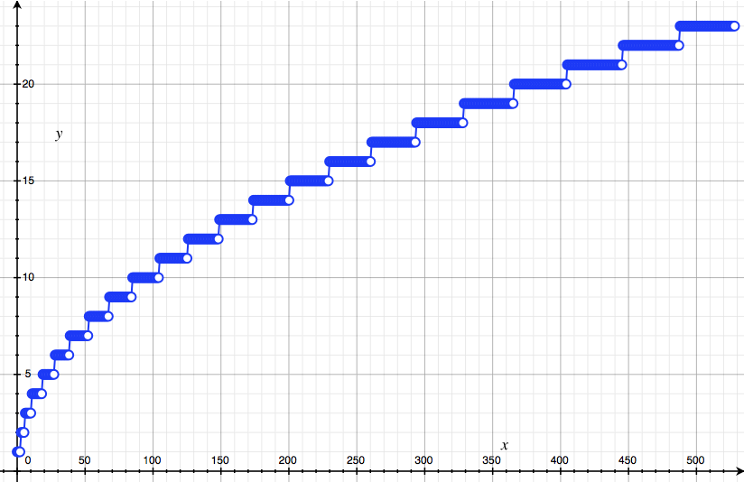
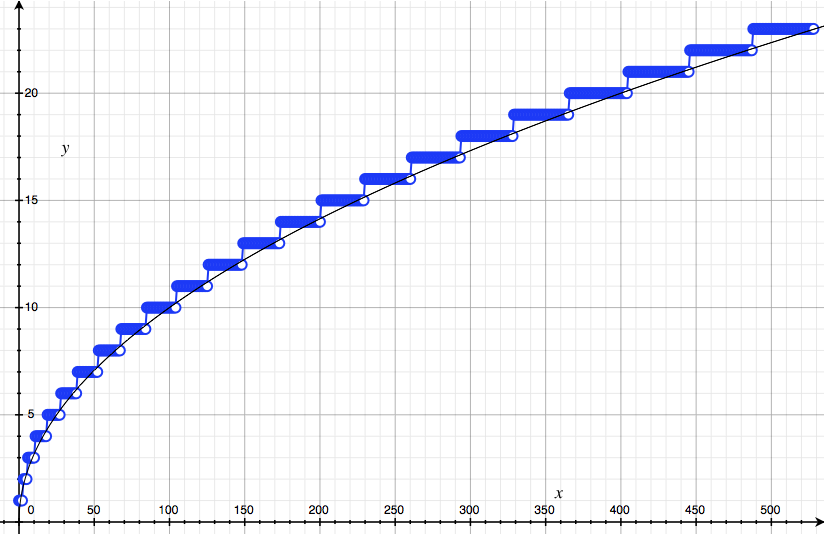
\[C_n \approx \sigma \sqrt{2\pi}.\]

(c) It remains for us to estimate $\sigma$, the standard deviation of this putative Bell curve. Write some code that takes $n$ and outputs $k_\sigma(n)$, the first point $k_\sigma \geq$ such that $a_{k_\sigma} \leq 0.6 a_n$. Calculate $k_\sigma(n)$ up until $n = 500$ or so and plot your results. They should look the picture below.

(d) The relationship is definitely not linear! To see what it is, plot the points on a log-log plot, and fit a straight line to the data. You should get something like:

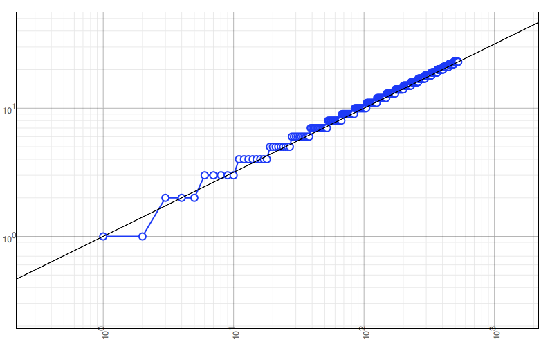
(e) Let $Y = \log y$ and $X = \log x$. Show that if $Y = mx$ on a log-log plot, then

\[y = x^m.\]

(e) From your answer to (d), or my plot, deduce that $m = 1/2$, and hence to a good approximation,

\[k_\sigma(n) \approx \sqrt{n}.\]

In case you’re suspicious, here is a plot $y = \sqrt{x}$ over the top of our data points:

(f) From this computationally-motivated guess for $k_\sigma(n)$, deduce that $C_n \approx \sqrt{2\pi n}$ and hence the improved Stirling approximation:

\[n! \approx \sqrt{2\pi n} \left(\frac{n}{e}\right)^n.\]

---

In case you’re wondering, the points $a_k$ really do describe an approximate Bell curve, and the approximation gets better as $n$ increases. This is because the rescaled points $p_k = e^{-n}a_k$ are examples of something called the Poisson distribution (also co-discovered by de Moivre!), with mean $n$ and standard deviation $\sqrt{n}$. They approach a Bell curve due to a major result from probability theory called the central limit theorem. Historically, though, the relation is the other way round. De Moivre found another way to get Stirling’s approximation, and used it to prove a special case of the central limit theorem for the Poisson distribution.

5. Euler’s formula

At this point, we are going to propose a remarkable reinterpretation of the exponential in the complex plane $\mathbb{C}$. In order to see how this comes about, we first have to review a few facts about complex multiplication. The one crazy idea, from which you can build everything else, is that there is some “imaginary” number $i$ such that $i^2 = -1$. A complex number has the form $z = x + iy$, where $x$ and $y$ are real numbers. We can picture these numbers as coordinates $(x, y)$ on the Cartesian plane. But unlike points on the Cartesian plane, there is now a natural way to multiply two complex numbers, based on $i^2 = -1$:

\[\begin{align*} z_1 z_2 & = (x_1 + iy_1)(x_2 + iy_2) \\ & = x_1 x_2 + i(x_1 y_2 + y_2 x_1) + i^2 y_1 y_2 \\ & = (x_1 x_2 - y_1 y_2) + i(x_1 y_2 + y_2 x_1). \end{align*}\]

This rule is a bit fiddly, but becomes much more transparent in polar coordinates. Recall that instead of specifying the $x$ and $y$ components, we can specify the angle $\theta$ (in radians) from the positive $x$ axis and distance $r$ from the origin. These give the $x$ and $y$ components using the usual rules of trigonometry:

\[\begin{align*} x & = r \cos \theta, \quad y = r \sin\theta \\ r & = \sqrt{x^2 + y^2}, \quad \theta = \tan^{-1}\left(\frac{y}{x}\right). \end{align*}\]

We denote the corresponding complex number $z(r, \theta)$. Let’s multiply two such complex numbers:

\[\begin{align*} z(r_1, \theta_1) z(r_2, \theta_2) & = r_1 (\cos\theta_1 + i\sin \theta_1) \cdot r_2 (\cos\theta_2 + i\sin \theta_2) \\ & = r_1 r_2 [(\cos\theta_1 \cos\theta_2 - \sin\theta_1 \sin\theta_2) + i (\cos\theta_1 \sin\theta _ 2 + \sin\theta_1 \cos\theta _ 2)]. \end{align*}\]

This still looks like a mess, but we can simplify dramatically using the compound angle formulas:

\[\begin{align*} \cos(\theta_1 + \theta_2) & = \cos\theta_1 \cos\theta_2 - \sin\theta_1 \sin\theta_2\\ \sin(\theta_1 + \theta_2) & = \cos\theta_1 \sin\theta _ 2 + \sin\theta_1 \cos\theta _ 2. \end{align*}\]

Applying these to $z(r_1, \theta_1)z(r_2,\theta_2)$ immediately gives

\[z(r_1, \theta_1) z(r_2, \theta_2) = r_1 r_2 [\cos (\theta_1 + \theta_2) + i \sin (\theta_1 + \theta_2)] = z(r_1 r_2, \theta_1+\theta_2).\]

In other words, a product of two complex numbers simply multiplies the lengths and adds the angles. Great! Now things can take an interesting “turn” (ahem). Without stopping to worry about justification, let’s plug an imaginary number into the exponential function, and use our formula for compound interest:

\[e^{i\theta} = \lim_{n\to\infty} \left(1 + \frac{i\theta}{n}\right)^n.\]

We know about complex multiplication, so we can understand $e^{i\theta}$ by analyzing the term in brackets:

\[z_n = 1 + \frac{i\theta}{n} = z_n(r_n, \theta_n).\]

Then the rules for multiplication give $e^{i\theta} = z(r_\infty, \theta_\infty)$, where

\[r_\infty = \lim_{n\to\infty} r_n^n, \quad \theta_\infty = \lim_{n\to\infty} n\theta_n.\]

From the formulas for converting from Cartesian to polar coordinates, we have a radius

\[r_n^2 = 1 + \frac{\theta^2}{n^2}.\]

When $n$ gets large, this is very close to $1$. In fact, you can prove in Exercise 5 that

\[r_\infty = \lim_{n\to \infty} r_n^{n} = 1.\]

So $e^{i\theta}$ lies a unit distance from the origin. The angle $\theta_n$ is a bit trickier. The conversion formula tells us that

\[\theta_n = \tan^{-1}\left(\frac{y_n}{x_n}\right) = \tan^{-1}\left(\frac{\theta}{n}\right).\]

For large $n$, $\theta/n$ is very small, so the small angle approximation $\tan^{-1} x \approx x$ tells us that

\[\theta_n \approx \frac{\theta}{n},\]

and this approximation becomes better and better as $n$ increases. But then

\[\theta_\infty = \lim_{n \to \infty} n\theta_n = \theta.\]

Hence, $e^{i\theta} = z(1, \theta)$, or

\[e^{i\theta} = \cos\theta + i \sin\theta.\]

This result was first derived by Swiss giant of mathematics Leonhard Euler, and thus goes by the soubriquet Euler’s formula. It is nothing short of a miracle that compound angles and compound interest are connected this way! As a special case, the formula yields an equation often said to be the most beautiful in mathematics:

\[e^{i\pi} = -1\]

since $\cos\pi = -1$ and $\sin\pi = 0$. There are many wonderful things Euler’s formula can do. We give two examples: de Moivre’s theorem in Exercise 6, and “infinite polynomials” for sine and cosine in Exercise 7.

---

Exercise 5. We will step through a (heuristic) proof that $r_\infty = 1$.

(a) Use the binomial theorem to show that

\[\left(1 + \frac{\theta^2}{n^2}\right)^n = 1 + \binom{n}{1}\left(\frac{\theta}{n}\right)^2 + \binom{n}{2}\left(\frac{\theta}{n}\right)^4 + \cdots + \binom{n}{n}\left(\frac{\theta}{n}\right)^{2n}.\]

(b) From this answer, deduce that the coefficient of $\theta^{2k}$, for $k \geq 1$, can be written

\[\frac{n!}{(n-k)!n^{k}} \cdot \frac{1}{n^k} \cdot \frac{1}{k!}.\]

(c) Use the fact that the first term approaches $1$ (which we argued above) to conclude that the whole term vanishes as $n\to\infty$. In other words, in the limit $n \to \infty$, only the first term of the infinite polynomial, namely $1$, survives. Hence, $r_\infty = 1$.

⁂

Exercise 6. As a special case of Euler’s formula, deduce de Moivre’s theorem,

\[(\cos \theta + i \sin\theta)^n = \cos(n\theta) + i \sin (n\theta).\]

Use this to find triple-angle formulas for $\cos(3\theta)$ and $\sin(3\theta)$.

⁂

Exercise 7. Let’s suppose that the infinite polynomial expression still holds for $e^{i\theta}$, so that

\[e^{i\theta} = p_\infty(i\theta) = 1 + i\theta + \frac{(i\theta)^2}{2!} + \cdots + \frac{(i\theta)^k}{k!} + \cdots.\]

Euler’s formula tells us that the real part of this formula is $\cos\theta$ and the imaginary part (multiplying $i$) is $\sin\theta$.

(a) By simplifying the factors of $i$ in $p_\infty(i\theta)$, argue that

\[\cos\theta = 1 - \frac{\theta^2}{2!} + \frac{\theta^4}{4!} + \cdots + \frac{(-1)^k\theta^{2k}}{(2k)!} + \cdots.\]

(b) Similarly, by consider the part proportional to $i$, argue that sine can be written as an infinite polynomial:

\[\sin\theta = \theta - \frac{\theta^3}{3!} + \cdots + \frac{(-1)^k\theta^{2k+1}}{(2k+1)!} + \cdots.\]

(c) Create numerical routines for $\cos\theta$ and $\sin\theta$, like you did for $e$ in Exercise 2.

---

6. Factorization and the Basel problem

In Exercise 7, we derived infinite polynomials for sine and cosine. Rather than repeat these derivations, let’s simply find the first two terms for sine. First, we notice that

\[e^{i\theta} = 1 + i\theta + \frac{i^2\theta^2}{2} + \frac{i^3\theta^3}{6} + \cdots = 1 + i\theta - \frac{\theta^2}{2} - \frac{i\theta^3}{6} + \cdots.\]

Since $e^{i\theta} = \cos\theta + i \sin\theta$, the terms proportional to $i$ must organize into some sort of infinite polynomial for $\sin\theta$. The first few terms are

\[\sin \theta = \theta - \frac{\theta^3}{6} + \cdots\]

There are two ways of writing ordinary polynomials: expanded and factorized. For instance, when we write

\[-2 - x + x^2 = (x - 2)(x+1),\]

we have the expanded form on the left and the factorized form on the right. We will boldly follow Euler and assume that this can sometimes be done for infinite polynomials as well! Recall that if a polynomial $p(x)$ has factorized form

\[p(x) = C(x - a_1)(x-a_2) \cdots (x - a_n),\]

then it equals zero precisely at $x = a_1, a_2, \ldots, a_n$. We know that $\sin\theta$ equals zero at

\[\theta = 0, \pm \pi, \pm 2 \pi, \pm 3\pi, \ldots.\]

This suggests that the infinite polynomial can be factorized as

\[\sin\theta = C \theta (\theta - \pi) (\theta + \pi) (\theta - 2\pi) (\theta + 2\pi) \cdots.\]

This vanishes at the right places, but we still need to determine $C$. With a bit of ingenuity, we can just take $\theta \ll 1$, and use the first term in the expanded form, $\sin\theta \approx \theta$. When $\theta \ll 1$, then in each factor $\theta \ll \pm k \pi$, and hence

\[\sin\theta = C \theta (\theta - \pi) (\theta + \pi) \cdots \approx \theta C(-\pi)(+\pi) (-2\pi)(+2\pi) \cdots.\]

To get this to equal $\theta$, we simply make the choice

\[C =[(-\pi)(+\pi) (-2\pi)(+2\pi) \cdots]^{-1}..\]

It seems $C$ has to be infinite! But assuming we can do this, we end up with

\[\begin{align*} \sin\theta & = C \theta (\theta - \pi) (\theta + \pi) (\theta - 2\pi) (\theta + 2\pi) \cdots \\ & = \theta \frac{(\theta - \pi)}{-\pi} \frac{(\theta + \pi)}{\pi} \frac{(\theta - 2\pi)}{-2\pi} \frac{(\theta + 2\pi)}{2\pi} \cdots \\ & = \theta \left(1-\frac{\theta^2}{\pi^2}\right) \left(1-\frac{\theta^2}{4\pi}\right) \left(1-\frac{\theta^2}{9\pi}\right) \cdots. \end{align*}\]

Though we have arrived by a slightly suspect route, this formula can be proved formally, though as usual we will not do so. Nifty as it is, we have not factorized for its own sake, but in order to do something even cooler. We just matched up the first term in the expanded polynomial for $\sin\theta$, and its factorized form, in order to figure out $C$. What about the next term? This is $-\theta^3/6$. In factorized form, we have an unavoidable factor of $\theta$ out the front, so it is going to be given by the quadratic term (proportional to $\theta^2$) when we expand

\[\left(1-\frac{\theta^2}{\pi^2}\right) \left(1-\frac{\theta^2}{4\pi}\right) \left(1-\frac{\theta^2}{9\pi}\right) \cdots.\]

Just like with the binomial theorem, we can think of this in terms of the choices we can make to get terms like $\theta^2$. Since each factor contains a multiple of $\theta^2$ or $1$, we can only choose it once! In every other factor we have to choose $1$. If we choose the $\theta^2$ term in the first factor, we get

\[\left(1-\frac{\theta^2}{\pi^2}\right) \to -\frac{\theta^2}{\pi^2}\]

and $1$ from everything else. If instead we choose the $\theta^2$ from he second factor, we get

\[\left(1-\frac{\theta^2}{4\pi^2}\right) \to -\frac{\theta^2}{4\pi^2}\]

and $1$ from everything else. In general, if we choose factor $k$, we will get a contribution $-\theta^2/(k\pi)^2$. So we will get a term

\[\frac{\theta^2}{\pi^2}\left(1 + \frac{1}{4} + \frac{1}{9} + \cdots \right).\]

We are (laboriously) expanding the factorized form, so the results must match the term we got from the exponential. Adding the $\theta$ back in, this means

\[\frac{\theta^3}{\pi^2}\left(1 + \frac{1}{4} + \frac{1}{9} + \cdots \right) = -\frac{\theta^3}{6},\]

and hence

\[1 + \frac{1}{4} + \frac{1}{9} + \cdots = \frac{\pi^2}{6}.\]

The problem of summing these reciprocal squares was posed in 1650 by Italian mathematician Pietro Mongoli, and solved 85 years later by a young Euler. It is called the Basel problem in honor of Euler, and the famous Bernoulli tribe of mathematicians who made valiant but unsuccessful attempts to crack Mongoli’s chestnut.

---

Exercise 8. Now it’s time to do it yourself!

(a) Find an infinite product form for $\cos\theta$.

(b) By matching the coefficients of $\theta^2$, argue that the sum of reciprocals of odd numbers is

\[1 + \frac{1}{3^2} + \frac{1}{5^2} + \cdots = \frac{\pi^2}{8}.\]

(c) Show that (b) also follows from the sum of reciprocal squares.

---

7. Ramanujan’s mysterious sum*

Euler’s results, as miraculous as they seem at first glance, follow from straightforward if slapdash manipulations. But the following chestnut is so miraculous it appears blatantly wrong:

\[1 + 2 + 3 + 4 + \cdots = -\frac{1}{12}.\]

It is a paradox. The sum of all the positive natural numbers is apparently not only finite, but negative! Although it seems like it cannot possibly be true, there is a rigorous way to interpret this statement so that is not only mathematically correct but useful. Some speculate that Euler may have known about it, but the first person to write it down and clearly understand it was Indian mathematician Srinivasa Ramanujan. Our approach, which differs slightly from Ramanujan’s, is the one used by physicists, and we will focus on its “physical” meaning.

We need one more elementary fact to get started. Recall the geometric series, stating that if $|r| < 1$, then the sum of its powers is

\[1 + r + r^2 + r^3 + \cdots = \frac{1}{1-r}.\]

The argument, if you haven’t seen it, is simplicity itself. Let $s$ be the series. Then

\[s - 1 = r + r^2 + r^3 + \cdots = r (1 + r + r^2 + \cdots ) = rs \quad \Longrightarrow \quad s = \frac{1}{1-r}.\]

Now we can begin our magic show. First, set $r = e^{-x}$ in the geometric series:

\[s_x = 1 + e^{-x} + e^{-2x} + e^{-3x} + \cdots = \frac{1}{1-e^{-x}}.\]

Consider a small change, $x \to x + \delta$ for $\delta \ll 1$:

\[s_{x+\delta} = 1 + e^{-(x+\delta)} + e^{-2(x+\delta)} + e^{-3(x+\delta)} + \cdots = \frac{1}{1-e^{-(x+\delta)}}.\]

To compare to $s_x$, we can use the formula for small changes:

\[e^{-kx} - e^{-k(x+\delta)} \approx k \delta e^{-kx}.\]

Hence, we can write

\[s_{x} - s_{x+\delta} \approx \delta e^{-x} + 2 \delta e^{-2x} + 3 \delta e^{-3x} + \cdots.\]

This sum looks potentially helpful, since the natural numbers now appear out the front of the exponential powers. But to evaluate the LHS more explicitly, we can sum the two geometric series:

\[\begin{align*} s_{x} - s_{x+\delta} & = \frac{1}{1-e^{-x}} - \frac{1}{1-e^{-(x+\delta)}}\\ & = \frac{e^{-x}-e^{-(x+\delta)}}{(1-e^{-x})(1-e^{-(x+\delta)})} \\ & \approx \frac{\delta e^{-x}}{(1-e^{-x})(1-e^{-(x+\delta)})}. \end{align*}\]

Equating our two expressions, dividing by $\delta$, and setting $\delta = 0$ (where the approximation becomes exact) we get the equation

\[\frac{e^{-x}}{(1-e^{-x})^2} = e^{-x} + 2 e^{-2x} + 3 e^{-3x} + \cdots.\]

To get the sum of natural numbers on the RHS, we would like to take $x \to 0$, so that $e^{-x} = 1$. On the LHS, the denominator will go to zero, so the whole expression will blow up, which is what we expect. But we will do this a bit more carefully, keeping track of powers of $x$. First, observe that

\[1 - e^{-x} = 1 - \left(1 - x + \frac{x^2}{2} - \frac{x^3}{6} + \cdots \right) = x\left(1 - \frac{x}{2} + \frac{x^3}{6} + \cdots\right),\]

and hence, using the geometric series in reverse,

\[\begin{align*} \frac{1}{1 - e^{-x}} & = \frac{1}{x\left(1 - x/2 + x^2/6 \cdots\right)} \\ & = \frac{1}{x}\left[1 + \left(\frac{x}{2} - \frac{x^2}{6}\right) + \left(\frac{x}{2} - \frac{x^2}{6}\right)^2 + \cdots\right] \\ & = \frac{1}{x}\left[1 + \frac{x}{2} - \frac{x^2}{6} + \frac{x^2}{4} + \cdots\right] = \frac{1}{x}\left[1 + \frac{x}{2} + \frac{x^2}{12} + \cdots\right]. \end{align*}\]

Finally, we can combine all these terms together in the expression

\[\begin{align*} \frac{e^{-x}}{(1-e^{-x})^2} & = \frac{1}{x^2}\left(1 - x + \frac{x^2}{2} + \cdots\right)\left(1 + \frac{x}{2} + \frac{x^2}{12} + \cdots\right)^2. \end{align*}\]

Multiplying out all the terms in brackets (or using WolframAlpha), we find that

\[\begin{align*} \frac{e^{-x}}{(1-e^{-x})^2} & = \frac{1}{x^2}\left(1 -\frac{x^2}{12} + \cdots \right) = \frac{1}{x^2} - \frac{1}{12} + \cdots. \end{align*}\]

where the $\cdots$ stand for positive powers of $x$. So, all in all, we have

\[e^{-x} + 2 e^{-2x} + 3 e^{-3x} + \cdots = \frac{1}{x^2} - \frac{1}{12} + \cdots.\]

As we take $x \to 0$, $e^{-kx} \to 1$ and hence the LHS gives us the sum of natural numbers. On the RHS, the powers of $x$ in the $\cdots$ vanish, but the $-1/12$ survives. Of course, there is also a term $1/x^2$, which blows up and gives us the infinity we expect. So why do physicists tend to ignore it? Consider $x \approx 1/N$ for a large number $N$. Then $e^{-kx}$ is close to $1$ until around $k \approx N/100$, since

\[e^{-N/100N} = e^{-1/100} \approx 0.99.\]

Terms below $N/100$ contribute to the sum, while terms above it are slowly but surely ignored, since they are multiplied by an exponential which goes to zero much faster than they increase. So we can think of the series

\[e^{-1/N} + 2 e^{-2/N} + 3 e^{-3/N} + \cdots\]

as the sum of natural numbers, but with terms above $N/100$ gradually ignored. To a physicist, we must ignore these large terms to get a sensible, finite answer, but the choice of $N$ is an arbitrary one without physical meaning. So, in the identity

\[e^{-1/N} + 2 e^{-2/N} + 3 e^{-3/N} + \cdots = N^2 - \frac{1}{12} + \cdots,\]

there is nothing meaningful about the $N^2$ on the RHS. It reflects an arbitrary choice about how to discipline a badly behaved sum, which forces it to tell us its true value. That true value is the term independent of $N$, namely $-1/12$. This is what physicists mean by

\[1 + 2 + 3 + 4 + \cdots = -\frac{1}{12},\]

no more and no less.

---

Exercise 9. We can use this approach to evaluate other crazy sums.

(a) Using Ramanujan’s sum, give a simple argument that

\[1 - 2 + 3 - 4 + \cdots = \frac{1}{4}.\]

(b) Without using Ramanujan’s sum, repeat the arguments from this section to evaluate

\[1 e^{-x} - 2 e^{-2x} + 3 e^{-x} - \cdots + (-1)^{k+1} k e^{-kx} + \cdots\]

and hence provide a rigorous interpretation of (a).

---

Acknowledgments

Thanks to J.A. for inspiring discussions. Section 7 is loosely based on Joe Polchinski’s textbook String theory. To my knowledge, the arguments in Sections 4 and 5 are original. The rest I have cribbed from sources beyond my power to recall.