December 23, 2020. Buffon asked how likely it is that a needle thrown onto ruled paper will cross one of the lines. The 1860 solution of Barbier is well-known. Equally simple but less well-known are the extensions to noodles and shapes of constant width, which I discuss informally, as well as a fanciful application to polymers.

Buffon’s needle

Suppose we throw a needle of length $\ell$ onto an infinitely large page, with lines ruled horizontally with separation $D$. If the needle is short, with $\ell < D$, it can cross at most one line. How likely is this? Following Joseph-Émile Barbier, we can split the randomness into two parts: the vertical position $y$ of the needle’s lower end, and it’s angle to the horizontal, $\theta$.

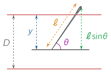
We therefore take $y \in [0, D)$, and $\theta \in [0, \pi)$. To see what the probability of hitting a line is, we note that the lower end of the needle will reach the upper line provided

\[y \leq \ell \sin \theta.\]

It’s easy to see that, assuming the parameters $(\theta, y)$ for the random throw take a uniform distribution in the rectangle below, the probability is just the area of the region below the line $y \leq \ell \sin \theta$, divided by the total area of the rectangle, $\pi D$.

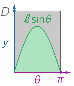
The area $H$ below the line (green) can be calculated using calculus:

\[H = \int_0^{\pi} \ell \sin \theta \, \text{d}\theta = \left[-\ell \cos\theta\right]^\pi_0 = \ell (\cos 0 - \cos \pi) = 2\ell.\]

There is another very simple way to see this without using calculus. Suppose you swing a slingshot around so that it executes a full revolution every $2\pi$ seconds. If the circle has radius $\ell$, the velocity (calculated by consider a full revolution) is

\[v = \frac{\text{distance}}{\text{time}} = \frac{2\pi \ell}{2\pi} = \ell.\]

The velocity has two sinusoidally varying components: a horizontal component, $v_x = \ell \sin \theta$ and a vertical component $v_y = \ell \cos \theta$.

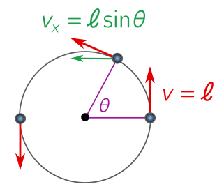
The horizontal velocity is exactly the curve of interest. The region underneath the curve is the total horizontal distance covered in half a revolution, since we are adding contributions of the form

\[v_x \, \Delta \theta = v_x \, \Delta t \approx \Delta x.\]

But if we add up all the small changes $\Delta x$ in a half-revolution, the total horizontal distance $H$ is obviously twice the radius, or $H = 2\ell$. No need for calculus! Either we get there, the probability that the short needle hits the line is

\[P = \frac{2\ell}{\pi D}.\]

Long needles and noodles

The above reasoning only works for short needles ($\ell < D$). When $\ell > D$, the green curve will exceed the grey rectangle, and the part outside does not contribute to the probability. We can calculate its area and subtract, but its a bit tedious. Let’s see what we can do with the result we already have. First, we can reformulate it a little. Let $N$ be the number of times a short needle hits a line. Our work above shows that the expectation is

\[\langle N \rangle = 0 \cdot P(N = 0) + 1 \cdot P(N = 1) = P(N = 1) = \frac{2\ell}{\pi D}.\]

Let’s now consider a long needle, with $\ell > D$. We can break it into some number of segments, say $n$, such that each is shorter than $D$, with length $\ell_i$. Let $N_i$, $i = 1, 2, \ldots, n$, label the number of times that segment $i$ hits a line, and $N$ the total number of lines that the long needle hits. Then we have

\[N = N_1 + N_2 + \cdots + N_n,\]

and hence, by the linearity of averages and our results for short needles,

\[\begin{align*} \langle N \rangle & = \langle N_1\rangle + \langle N_2 \rangle + \cdots + \langle N_n \rangle \\ & = \frac{2\ell_1}{\pi D} + \frac{2\ell_2}{\pi D} + \cdots + \frac{2\ell_n}{\pi D} \\ & = \frac{2(\ell_1 + \ell_2 + \cdots + \ell_n)}{\pi D} = \frac{2\ell}{\pi D}. \end{align*}\]

What do you know! The formula for the expected number of crossings is the same, even though the probabilities change.

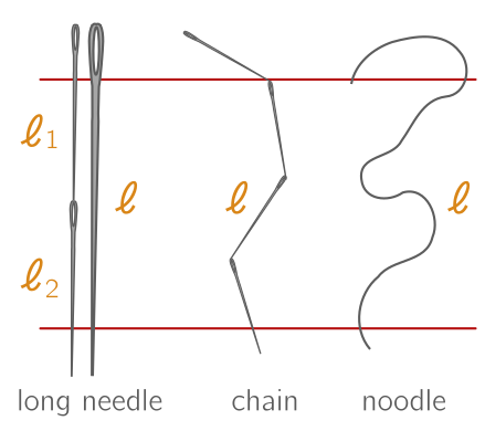
But something even more remarkable is true. This result was independent of the relative orientation of the segment, so it holds for a chain of line segments which twists and turns. And in fact, we can take the limit of $n \to \infty$, so that our curve becomes smooth, without affecting our formula. We conclude that, for an arbitrary plane curve of length $\ell$ (such as a noodle), the expected number of crossings is

\[\langle N \rangle = \frac{2\ell}{\pi D}.\]

This result is also due to Barbier, but credit for “Buffon’s noodle” goes to J. F. Ramaley.

Woodles

The final twist of the noodle comes from thinking about shapes which have constant width. Consider a circle of radius $r$ for instance. However you choose to orient it, it will have a width of $2r$, in the sense that you cannot pass it through a gap any smaller, and you can always pass it through a wider gap. If we happen to rule lines at a distance of $D = 2r$, then a randomly thrown circle will have exactly two crossings, with the same line piercing the circle twice, or two lines just tangent to the circle at the top and bottom.

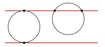
We can check this previous noodle result, note that the expected number of crossings is

\[P = \frac{2 \ell}{\pi D} = \frac{2 \cdot 2\pi r}{\pi \cdot 2 r} = 2.\]

But we can go in the other direction. Suppose that a shape has constant width $D$, so however it is oriented, it has exactly two crossings when lines are ruled with spacing $D$. Then the perimeter $\ell$ is twice the width:

\[P = \frac{2 \ell}{\pi D} = 2 \quad \Longrightarrow \quad \ell = \pi D.\]

This result is called Barbier’s theorem. Constant width surfaces are fun because they can replace circles as wheels, at least if they are allowed to simply roll along underneath a flat surface, the way that Egyptians and Romans moved building materials on logs. (The centre of any of these non-circular constant width curves wobbles up and down, so they are less useful if you are using axles. But this is not an insurmountable obstacle.) Since “wheels” suggests circles, and “constant-width shape” is cumbersome, I’ll call non-circular constant-width shapes “woodles” for “wheely noodles”.

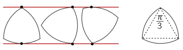
Above, I’ve shown a woodle called the Reuleaux triangle after the German engineer Franz Reuleaux. It’s a beautiful shape, created by starting with an equilateral triangle, then rotating one edge until a corner until it hits another, subtending $\pi/3$ of a circular arc. The width is simply the side length of the triangle $D$, and we are dragging out $(\pi/3) D$ a total of three times, so the perimeter $\ell = \pi D$ as expected.

I could write a whole post on this shape and its many uses (and maybe I will!) but instead, I’ll briefly mention that the Reuleaux construction can be generalized to an odd-sided regular $s$-gon, replacing sides with arcs of a circle pivoting around the opposite corner. (If it’s even-sided, the arcs you attempt to draw will lie inside the polygon.) The width is simply the side length $D$ of the polygon, and the same reasoning shows that we draw arcs subtending $(\pi/s)D$ a total of $s$ times, so $\ell = \pi D$ as Barbier’s theorem tells us.

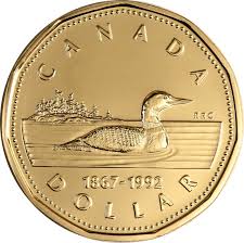
Two practical application of constant-width Reuleaux polygons are to manhole designs and coinage. Manholes apparently need to be constant width so they don’t turn and fall through the hole. In fact, this is a famous interview question for Microsoft! As discussed by Tanya Khovanova, this isn’t quite true in general, since they only need to not fall through the hole, i.e. the minimum width of the cover exceeds the maximum width of the hole. Turning to coins, coin-operated machines can use any constant-width shape, so they can be more general than a circle. This leads to a fun little piece of mathematical Canadiana: the loonie (one dollar coin) is not a circle, but an 11-sided Reuleaux woodle!

Random noodles and polymers

Although the expected number of crossings is easy, in general, for a fixed curve the actual probability distribution for $N$ is complicated. But things simplify for a random noodle made of independent random steps. A physical example is a polymer, the long jointed molecules making up plastics or DNA, or the path traced out in time by particles in a fluid. Suppose the noodle is made from $n$ straight segments of length $\ell_i < D$ and total length $\ell$. Then each segment represents an independent “trial”, and the joint distribution is multinomial. In the special case that the step lengths are the same, $\ell_i = \lambda$, then the number of crossings obeys a binomial distribution $\mathcal{B}(n, P)$ for $P = 2\ell/\pi D$. This has mean $\langle N\rangle = nP$ as we already calculated, and standard deviation

\[\sigma^2 = n P (1 - P).\]

But we can actually give the probabilities explicitly:

\[P(N = k) = \binom{n}{k}P^k (1- P)^{n-k}, \quad P = \frac{2\lambda}{\pi D}.\]

Since $\langle N\rangle = nP$ is the expected number of crossings, in the limit that we keep this expectation fixed but take $n \to \infty$, i.e. a continuous random noodle, the De Moivre-Laplace theorem (a special case of the central limit theorem) tells us that the distribution will converge to a normal:

\[\mathcal{N}(\mu, \sigma^2), \quad \mu = nP, \quad \sigma^2 = nP(1-P).\]

In physical examples like a polymer, however, it’s more realistic to treat $\lambda$ as a finite persistence length (or technically Kuhn length). Throwing the chains many times gives a fanciful means of estimating persistance length, since after many trials, the sample mean $\bar{\mu}$ and sample variance $\bar{\sigma}^2$ obey

\[\lambda = \frac{\pi D}{2}\left(1 - \frac{\bar{\sigma}^2}{\bar{\mu}}\right).\]

There are various impracticalities with this scheme. But that shouldn’t spoil the fun of applying Buffon’s noodle to the microphysics of polymers!