January 26, 2021. The bus paradox states that, if buses arrive randomly but on average every ten minutes, the expected waiting time is ten minutes rather than five. I give a simple proof involving no integrals or formal probability theory.

Introduction

The bus paradox (also called the waiting time or inspection paradox) is a counterintuitive result about waiting times between random events. Suppose buses arrive randomly, with an average period of $\lambda$ between arrivals. If you go to catch a bus, you might expect to wait a period $\lambda/2$, since if a bus arrives $\lambda/2$ after you arrive, and $\lambda/2$ before you arrive (by symmetry), then the gap between them is $\lambda$. This reasoning is wrong, and rather unexpectedly, the expected wait time is $\lambda$. The goal of this post is to give a proof which does not require any integrals or formal probability theory, and makes the role of assumptions manifest.

The bus loop

We start by considering a circle of total length $L$, on which we place $k$ points at random (white in the image below). This models a length of time, such as the day, and the random arrival of $k$ buses. The average distance between points (going clockwise, for instance) is clearly

\[\lambda = \frac{L}{k}.\]

Let us place another point on the circle at random (black in the image below). This represents the commuter who wishes to catch a bus.

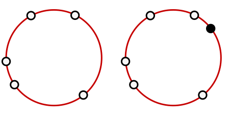
Since we now have $k + 1$ points placed at random, the same reasoning as above tells us that the average distance is

\[\frac{L}{k +1} = \left(\frac{k}{k+1}\right)\lambda.\]

Translating into the language of bus schedules, this means that if buses have a fixed but random schedule over some length of time, with average interarrival time $\lambda$, the expected wait time is not $\lambda$, but rather, smaller than $\lambda$ by a factor of $k/(k+1)$, where $k$ is the total number of buses over the period.

The bus paradox

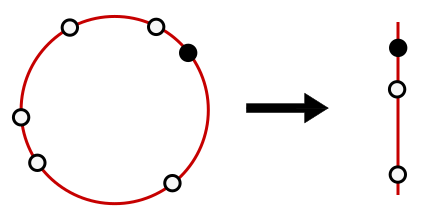
The bus paradox applies to a schedule which does not repeat. Let us take $L, k \to \infty$ but leave $\lambda = L/k$ fixed. We represent this by an infinitely large circle, with a straight edge, in the image below. Then the expected waiting time is

\[\left(\frac{k}{k+1}\right)\lambda \to \lambda.\]

Thus, the arrival of the commuter is equivalent to adding another random bus. The corresponding interarrival period is modified, but by a vanishingly small coefficient as $k \to \infty$. This completes our simple proof of the bus paradox.

It’s a little tricky, of course, to formulate what it means to place the buses “uniformly” on an infinite line, and this is exactly what the Poisson process (and more generally renewal theory) achieves. But rather than introduce all this formal baggage, we can simply consider the limit of the uniform process to arrive at the correct conclusion, and with greater clarity than when the answer is concealed in thickets of algebra.

Conclusion

The reasoning outlined in the introduction is not completely off the mark. It applies when the buses arrive at fixed intervals $\lambda$, and the commuter randomly. The expected time to the previous bus $t_-$ and the expected time to the next bus $t_+$ must add to give the interval $\lambda$ between buses, and by time symmetry, they must be equal:

\[t_+ + t_- = \lambda, \quad t_+ = t_- \quad \Longrightarrow t_+ = t_- = \frac{\lambda}{2}.\]

In this case, there is a clear distinction between the stochasticity of buses and commuters. But when everything arrives randomly, a commuter becomes like just another bus.