September 8, 2018. Getting a handle on higher-dimensional objects is hard. In very high dimensions, however, we can view simple shapes as random processes, and convert statistical properties into geometric ones. I’ll explore this approach for hypercubes, loosely speaking the geometry of coin flips.

Introduction

Prerequisites: undergraduate probability.

Visualising things clearly in three dimensions is hard enough, and it’s what our brains were designed for. Imagining higher spatial dimensions seems almost impossible! For four spatial dimensions, there is a trick: pretend that the additional dimension is time. For instance, you could think of a 4-dimensional cube as a regular cube which pops into existence, sits there for a second, then disappears again. If somebody records a video of the cube with 3D goggles, we have a “graph” of the cube in four dimensions. In other words, we convert a process (the popping into and out of existence) into geometry.

Although it helps us visualise a 4-dimensional cube, the analogy does not yield any real insights into the geometric properties. In fact, it’s misleading! Special relativity teaches us that time is just another dimension, sure, but one which is fundamentally different from the spatial directions. This is captured by the fact that you can’t travel faster than light.

However, it turns out that a version of this trick — geometrising a process — works for $n$ dimensions, where $n$ is much larger than $1$. Although we can’t directly visualise a million-dimensional space this way, the process viewpoint encodes some deep insights into higher-dimensional shapes. Roughly speaking, shapes are like probability distributions, dimensions are samples from these distributions, and the behaviour of many data points is much simpler than the behaviour of a few.

Hypercubes

We’re going to focus on the simplest family of higher-dimensional shapes: the hypercube, a generalisation of the cube. Examples are the unit interval $I=[0,1]\subseteq \mathbb{R}$, the unit square $I\times I=I^2\in {\mathbb{R}}^2$, the cube $I^3\subseteq {\mathbb{R}}^3$, and the tesseract $I^4\subseteq {\mathbb{R}}^4$, pictured below.

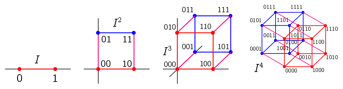
We build the square $I^2$ by taking two copies (red and blue) of the interval $I$, placing them a unit distance apart in a new orthogonal direction, and joining them up (purple). We build the cube by joining two copies of the square, and the tesseract by joining two copies of the cube. Hopefully you get the idea: to construct $I^{n+1}$, put two copies of $I^n$ a unit distance apart in a new dimension orthogonal to all the others, and join them up. Thus, we can explicitly write

$$I^n=\{\mathbf{x}=(x_1,x_2,\cdots ,x_n):x_i\in [0,1]\}.$$

This way of constructing a hypercube $I^n$ can be turned around and used to deconstruct a hypercube. The full hypercube is an $n$-dimensional object, the unique $n$-dimensional “face”. On the other end of the spectrum are the corners, which are $0$-dimensional objects we can think as “$0$-faces”, or copies of the $0$-cube $I^0$, consisting of a single point. There are $2^n$ corners, since at a vertex each coordinate $x_i$ must be $0$ or $1$; since there are $n$ such choices to independently make, the total number is

$$\stackrel{n\text{ times}}{\overbrace{2\times 2\times \cdots \times 2}}=2^n.$$

More generally, if we choose $0\le k\le n$ coordinates to be “extreme”, i.e. at $0$ or $1$, we are left with a copy of the $(n-k)$-cube. Thus, there are $2^k$ $(n-k)$-faces, or relabelling $k\leftrightarrow n-k$, there are $2^{n-k}$ copies of each $k$-face. The $k$-faces are labelled by binary strings $s_{n-k}$ of length $n-k$, corresponding to the choice of $n-k$ extreme coordinates.

(Note that I’ve defined $k$-faces with respect to a specific ordering of dimensions, and they all end up being parallel. I’ll call these ordered $k$-faces. More generally, a $k$-face is obtained by choosing any subset of $n-k$ dimensions to make extreme; these are general $k$-faces. These are a bit less nice, since they do not decompose the hypercube.)

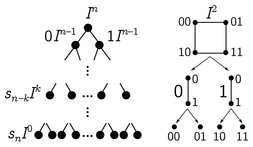
To summarise, our technique for iteratively constructing hypercubes can be used to deconstruct $I^n$ into a binary tree of hypercubes of lower dimension. We won’t really exploit this fact below, but it gives us another way to understand higher-dimensional structure.

Random corners

Let’s look at the corners in more detail. These are labelled by $n$-bit strings, i.e. any sequence $s_n$ of $1$s and $0$s of length $n$ corresponding to the taking the usual $n$-tuple notation and throwing away commas and brackets, e.g. $(0,1,1,0,1)\mapsto 01101$. Binary strings appears all over the place, but in probability, they usually represent a sequence of Bernoulli trials, i.e. the result of flipping a coin. This means I can pick a corner of the hypercube uniformly at random by flipping a fair coin $n$ times, and statistical properties of this random process will encode geometric properties of the corners. Put a different way, the hypercube makes the space of $n$ coin flips geometric.

The cleanest example is the average distance from the origin. Recall that in ${\mathbb{R}}^n$, the distance of a point $\mathbf{x}=(x_1,x_2,\cdots ,x_n)$ from the origin is

$$d=|\mathbf{x}|=\sqrt{x_1^2+x_2^2+\cdots +x_n^2}.$$

For the corners of a cube, things are even simpler: if a corner has $a$ $1$s and $b$ $0$s in some order, then the distance is simply $d=\sqrt{a}$. Imagine that we pick a corner of the hypercube $I^n$ by flipping a fair coin $n$ times, assigning $0$ to heads and $1$ to tails. If $n$ is very large, we should get roughly the same number of heads and tails, so

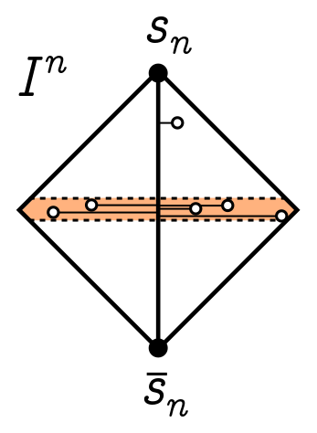
$$a\approx b\approx \frac{n}{2}⟹d\approx \sqrt{\frac{n}{2}}.$$

For a high-dimensional hypercube, most corners are $\sqrt{n/2}$ away from the origin. But there is nothing special about the origin. Every other corner of the cube looks the same, so most corners are $\sqrt{n/2}$ from each other! So, pick any corner labelled by a binary string $s_n$, and consider the opposite corner ${\overline{s}}_n$, obtained by flipping all the bits in $s$. Let $s^{(i)}$ denote the $i$-th digit of the string $s$, and define the vector $\mathbf{x}(s)$ corresponding to a string $s$ by

$$x(s{)}_i=s^{(i)}.$$

The distance between $s_n$ from ${\overline{s}}_n$ is then

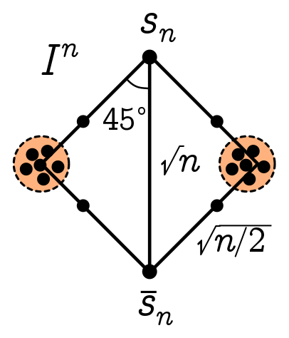
$$d(\mathbf{x}(s_n),\mathbf{x}({\overline{s}}_n))=|\mathbf{x}(s_n)-\mathbf{x}({\overline{s}}_n)|=\sqrt{\sum _{i=1}^n(s_n^{(i)}-{\overline{s}}_n^{(i)}{)}^2}=\sqrt{n},$$

since $(s_n^{(i)}-{\overline{s}}_n^{(i)}{)}^2=1$ by definition of the flipped string ${\overline{s}}_n$. Since the distance from $s_n$ (or ${\overline{s}}_n$) to most other corners is $\sqrt{n/2}$, the angle made between “long” diagonal from $s$ to $\overline{s}$, and most other points, is

$$\cos \theta =\frac{\sqrt{n}/2}{\sqrt{n/2}}=\frac{1}{\sqrt{2}}⟹\theta ={45}^{\circ }.$$

Thus, we get the cartoon geometry for the hypercube corners above.

Random interior points

If we wanted to, we could use similar techniques to study the geometry of $k$-faces. I’ll leave this to you to think about. Let’s go right to the top of the tree and study the distribution of interior points. Average distance turns out to be messy, so instead, we’ll look at the projection of a random interior point onto the long diagonal from $s$ to $\overline{s}$.

It will be simplest to just set $s=0^n$ and $\overline{s}=1^n$, with a diagonal

$$\ell =\stackrel{n\text{ times}}{\overbrace{(1,1,\cdots ,1)}},\hat{\ell }=\frac{1}{|\ell |}\ell =\frac{1}{\sqrt{n}}\stackrel{n\text{ times}}{\overbrace{(1,1,\cdots ,1)}}.$$

If we project a point $\mathbf{x}$ onto $\ell$, it will be a distance from the origin

$$\mathbf{x}\cdot \hat{\ell }=\frac{1}{\sqrt{n}}\sum _{i=1}^n{x}_i=\sqrt{n}\overline{x},$$

where $\overline{x}$ is the average of the coordinates $x_i$. Once again, let’s select an interior point $\mathbf{x}$ at random. This means we select each coordinate $x_i$ uniformly from $I=[0,1]$. Thus, we can view a random point $\mathbf{x}$ as drawing $n$ samples from the uniform distribution on $I$, and as $n$ gets large, the sample average of these points should approach the average of the distribution, $\mu =1/2$. Thus, the projection onto the long diagonal satisfies

$$\mathbf{x}\cdot \hat{\ell }=\sqrt{n}\overline{x}\to \frac{\sqrt{n}}{2}.$$

Since the diagonal has length $\sqrt{n}$, we learn that most points are near the halfway mark, as we drew above.

---

Exercise 1. (a) Show that two randomly chosen, ordered $k$-faces are separated by an average distance

$$\sqrt{\frac{n-k}{2}}.$$

Similarly, if two general $k$-faces are parallel in $j$ dimensions, show that the average distance is

$$\sqrt{\frac{j}{2}}.$$

(b) Show that for two randomly chosen, general $k$-faces, the probability of being parallel is

$${(\genfrac{}{}{0ex}{}{n}{k})}^{-1}.$$

Prove that the probability of being parallel in $j\le k$ dimensions is

$$(\genfrac{}{}{0ex}{}{n}{j,k-j,k-j,n-2(k-j)}){(\genfrac{}{}{0ex}{}{n}{k})}^{-2}.$$

(c) Write an expression for the average distance between general $k$-faces.

---

Chernoff bound for corners

So far, we have been pretty sloppy about the spread of corners and interior points around the mean values, or its inverse, the concentration. Let’s remedy this. We start with a simple application of the Chernoff bound, which states that for any random variable $X$, and any $t\in \mathbb{R}$,

$$\mathbb{P}(X\ge c)\le \frac{\mathbb{E}[e^{tX}]}{e^{ct}}.$$

Let $X=a$, the sum of digits in a random binary string $s_n$. I will leave it as an exercise to figure out what the bound gives us.

---

Exercise 2. (a) Recall that the binomial distribution is

$$\mathbb{P}(X=k)=2^{-n}(\genfrac{}{}{0ex}{}{n}{k}).$$

Show that the expectation satisfies

$$\mathbb{E}[e^{tX}]={\left(\frac{1+e^t}{2}\right)}^n.$$

(b) Define $c=n\alpha$, so that $\alpha$ describes the proportion of coordinates (or bits) equal to $1$. Show that the right-hand side of the Chernoff bound is optimised for

$$e^t=\frac{\alpha }{1-\alpha }.$$

(c) Plug this optimal value into the Chernoff bound to find

$$\mathbb{P}(\frac{X}{n}\ge \alpha )\le {\left\{{\left(\frac{\alpha }{1-\alpha }\right)}^{-\alpha }\frac{1}{2(1-\alpha )}\right\}}^n.$$

(d) Using part (c), show that the probability a random corner has more than $60\mathrm{\%}$ of its coordinates equal to $1$ is bounded by

$$\mathbb{P}(\frac{X}{n}\ge 0.6)\lesssim {0.98}^n.$$

How many dimensions do we need to go to before this probability is less than $0.01$?

---

Stragglers in high dimensions

The Chernoff bound gives us results for small $n$, but it is fiddly and underestimates the concentration. Rather than repeat the analysis for the interior points, we will make life simpler by going to very high dimensions. As $n\to \mathrm{\infty }$, there are two powerful results we can invoke: the law of large numbers and the central limit theorem. They are simple to explain, and not much harder to prove, though we will not do so here.

The (strong) law of large numbers states that as $n\to \mathrm{\infty }$, the sample mean

$${\overline{x}}_n:=\frac{1}{n}\sum _{i=1}^n{x}_i$$

for a set of independent, identically distributed random variables $x_i$ converges to the mean of the distribution, $\mu =\mathbb{E}[x_i]$:

$$\mathbb{P}(\underset{n\to \mathrm{\infty }}{lim}{\overline{x}}_n=\mu )=1.$$

This immediately tells us that as $n\to \mathrm{\infty }$, the corners and interior points are concentrated around the mean values we calculated above. Our earlier sloppiness has been morally vindicated! At any finite $n$ there may be stragglers, but these are a vanishing fraction of the whole.

If we want to know more about the stragglers at large but finite $n$, the central limit theorem is the tool of choice. This gives us the whole distribution of ${\overline{x}}_n$ as $n$ gets large. If we add $n$ independent copies of the same random variable $x_i$, the mean and variance of the sum are just multiplied by $n$ (since both are additive for independent random variables):

$$\mathbb{E}[{\hat{x}}_n]=\mu ,\mathrm{Var}[{\overline{x}}_n]=\frac{1}{n^2}\mathrm{Var}\left[\sum _i{x}_i\right]=\frac{{\sigma }^2}{n}.$$

Higher moments are suppressed by additional factors of $n$. As $n$ gets big, only the first and second moment survive, which is the characteristic of a normal distribution, or bell curve. We discover that

$${\overline{x}}_n\stackrel{n\to \mathrm{\infty }}{\sim }\mathcal{N}(\mu ,{\sigma }^2/n),$$

where $\mathcal{N}$ denotes the normal distribution.

To apply to our case, we need to compute the variance. For the corners, the $x_i$ are fair Bernoulli trials with variance $1/2$. Hence, as $n$ gets large, corners are normally distributed around the mean distance $\sqrt{n}/2$ with variance $1/2n$. For the interior points, the $x_i$ are uniformly distributed on $[0,1]$, which has variance

$${\int }_0^1{x}^{2}dx-{\left(\frac{1}{2}\right)}^2=\frac{1}{12}.$$

Thus, as $n$ gets large, interior points are concentrated in a Gaussian envelope around the bisecting plane, with variance $1/12n$.

Hinton’s anchovies

We’ve learnt that for hypercubes in higher dimensions, the corners and volume tend to concentrate around the mean values. The route we used to arrive at this conclusion was statistical, but turns out to be an instance of a much deeper phenomenon called concentration of measure. In some sense, concentration is generic.

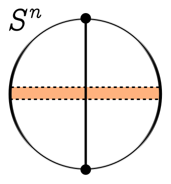
The most famous higher-dimensional shape is not the hypercube, but the $n$-dimensional hypersphere $S^n$, which generalises the sphere in the same way the hypercube generalises the cube. You can learn more about the details in the references below, but qualitatively, we see a similar concentration phenomenon. Selecting two antipodal points on the sphere (analogous to two opposite corners), the boundary and volume will cluster normally around the bisecting plane.

Although concentration is the deep explanation for what’s going on here, there is a nice intuition for why the hypercube and hypersphere look the way they do. I like to think of this as the anchovy phenomenon after a talk by Geoffrey Hinton. He first considers a three-dimensional supermarket, where anchovies are with the pizza toppings, rather than the tuna and canned sardines on the other side of the supermarket where he first looks. But you can have more neighbours in higher dimensions! As Hinton puts it,

…if it had been a thirty-dimensional grocery store, they could have been near the pizza and the sardines.

If we think of one corner as pizza toppings, and the opposite corner as sardines, most points on the hypercube are like anchovies.

References

• “Geometry in Very High Dimensions”, Renato Feres.
• Computer Science Theory for the Information Age (2012), John Hopcroft and Ravi Kannan.
• Intuitive crutches for higher dimensional thinking (2016), MathOverflow post.