January 20, 2021. Why are dice and coins good sources of randomness? The word “symmetry” is bandied about, but symmetry is not enough to explain why starting with very similar initial conditions and evolving deterministically leads to random outcomes. I explore the relevant factors—chaos and jitter—and use them to build deterministic dice.

Introduction

Each time I roll a dice, my muscles try to do the same thing. But even if I hold the dice the same way, and throw in what feels like the same way, I seem to get any side of the dice with equal probability. If you ask why a mathematician why any face is equally probable despite the apparent similarity of the roll, they might say symmetry. Apart from the pips indicating the value [¹], the sides are indistinguishable and therefore must have equal probability of landing right side up. This is true and sounds like a nice explanation. But it’s only half the story!

To see why, suppose I take a very large dice, so heavy that I can only drop it. In this case, it’s unlikely to roll, and whatever side happens to be facing up when I “roll” will be facing up when it stops [²]. If I pick this face randomly, I will get a random outcome, but the point of the dice is to outsource the randomness! Symmetry is important, as we will see, but using dice is fundamentally a roll-playing game.

The Butterfly Effect

To illustrate our ideas, we’ll use the even simpler example of flipping a coin. Once again, ignoring the small effect of markings, the coin has a symmetry between the two sides, heads and tails. And similarly, if I have a very large coin I can only drop, then I will need to randomly choose the initial conditions for tossing if I want the coin flip to be random. This defeats the purpose of the coin! So, how does a deterministic process like throwing a coin generate an effectively random and uniform outcome? There are two main ingredients, as I see it: chaos and jitter.

We’ll focus on chaos first, and a particular characterisation of chaos called the “butterfly effect”, aka sensitivity to initial conditions. Suppose a system has some space of configurations $\mathcal{C}$, with the specific configuration at any time $t$ denoted $x(t) \in \mathcal{C}$. We’ll restrict ourselves to systems which evolve according to some deterministic rule, i.e. the state $x(t)$ at time $t$ determines the state $x(t’)$ for any $t’ > t$ [³]. Finally, we imagine that $\mathcal{C}$ has a notion of distance between configurations, denoted by the absolute value sign, $|x_1 - x_2|$. Then the system is chaotic (in the butterfly sense) if the distance between nearby configurations increases exponentially with time:

Time here need not be continuous, but could come in discrete steps, with $t = 0, 1, 2, \ldots$. The rate of exponential divergence is controlled by $\lambda$, called the Lyapunov exponent after Aleksandr Lyapunov.

We can see how this operates in a very simple chaotic system called the doubling map. The configuration space $\mathcal{C} = [0, 1]$ is just the unit interval. Time is discrete, and at each step, we simply double the configuration and keep only the fractional part, denoted by “mod $1$”. So we can describe the system by

It’s easy to see this system is chaotic, since if we take two nearby points $x(0), y(0)$, then

provided the difference remains smaller than $1$. Thus, the Lyapunov exponent for this system is $\lambda = \log 2$.

Exploring configuration space

At some point the doubling means that the difference gets so large it is no longer doubling with each step, since we are throwing away whole numbers. To see how this happens, let’s do a specific example. Set $x_0 = 0.1$ and $y_0 = 0.2$. Then

This does not mean the butterfly effect has “stopped”. Rather, this is the point at which the effect has fanned the two trajectories out so they explore the whole system! We can estimate the time this happens as follows. Suppose the configuration space $\mathcal{C}$ has some effective linear size $L$, and chaotic evolution with Lyapunov exponent $\lambda$. Then two trajectories with initial separation $\ell$ should spread throughout the whole system in a time $T$ given by

In our example, $\ell = 0.1$ and $L = 1$, so

which is consistent with our discrete-time result $T = 4$.

We’ll call $T$ the exploration time, since this is roughly how long it takes for trajectories to fan out and explore the whole space. In fact, if we choose a collection of initial conditions in some region of size $\ell$, the exploration time should still tell us roughly how long elements of this set need to spread throughout all of configuration space. Because of chaos, unless we know precisely which trajectory we picked, predictability should totally break down, since initially nearby points (order $\ell$) are now separated by distances on the order of the whole system (order $L$). This breakdown leads to an effectively randomisation over configuration space.

Chaotic coins

This effective randomness is why we roll dice and throw coins. Symmetry is still important, since it splits the configuration space $\mathcal{C}$ into regions of equal size, into which chaos threads trajectories in a roughly uniform way. If the system doesn’t get to evolve for long enough, like dropping the large dice, trajectories don’t spread and the result is strongly biased by the initial conditions. But after a few exploration times, we should be equally likely to be in any of these symmetrically defined patches, when averaged over the initial conditions.

This sounds like a mathematical theorem, and perhaps there is something we can rigorously prove here. But technical results about probability, dynamics and mixing involve averaging over very long times, $T\to \infty$, rather than the exploration time we’ve introduced here, and I’m not sure what tools we could use [⁴]. Instead of proving a theorem, however, we can use our concepts to design coins and dice from scratch and check they behave correctly. We’ll just use the doubling map!

To start with, let’s make a coin [⁵]. Heads will correspond to $\mathcal{C}_H = [0, 0.5)$ and tails to $\mathcal{C}_T = (0.5, 1]$. We randomise the initial condition to lie in the interval $[0, \ell)$, evolve for some number of steps, then make a decision based on whether the current position is in $\mathcal{C}_H$ or $\mathcal{C}_T$. We can empirically compute the bias of our chaotic coin by repeating the experiment for random initial conditions some number of times, adding the number of tails, and dividing by the total number of experiments. Here is a plot for $\ell = 0.1$, with bias on the vertical axis and the number of exploration times on the horizontal axis:

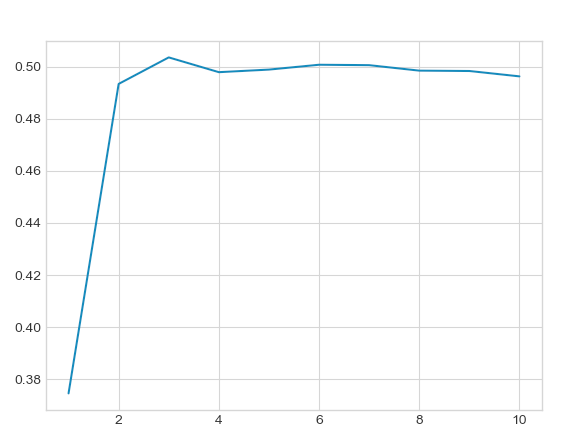
The code for generating this and subsequent plots is given in the appendix. It increases from highly biased towards heads (where our initial conditions start) to fair, after a few exploration times, just like we expect. There is nothing special about $\ell = 1$ either. Below, we plot the curves for $\ell = 0.001$ (black), $0.01$ (red), $0.1$ (blue), $0.5$ (orange):

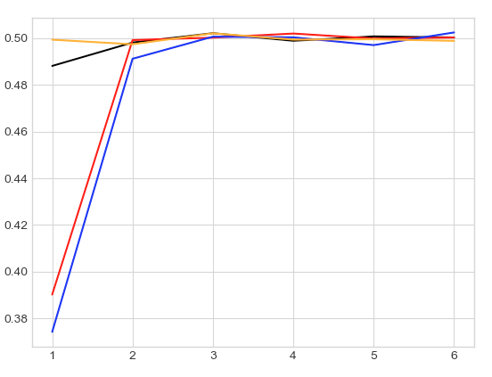
Although the curves look somewhat different when plotted in actual steps, they all approach fairness after a few exploration times.

Chaotic dice

Naturally, we can use the same method to create a dice. Instead of splitting the space into two equal halves, we split it into six equal portions, $\mathcal{C}_i$ for $i = 1, \ldots, 6$. In fact, it’s clear that we could do this for a coin with any number of sides! We’ll focus on six for simplicity. We proceed in exactly the same way, but now it’s a bit more complicated to check for bias, and we need to make a brief detour into statistics. As nicely explained in this post on the RPG stack exchange, the simplest check is the Pearson $\chi^2$ test. Suppose our dice has $d$ sides, and we want to check after some number of rolls how fair it appears to be. Let $N$ be the total number of observations, $N_i$ the number of observed rolls with value $i$, and $p_i = 1/d$ the uniform probability. Then the statistic

approaches a $\chi^2$ distribution with $d - 1$ degrees of freedom as the number of samples $N$ gets large [⁶]. Let’s plot the Pearson statistic for many ($N = 10^5$) rolls, and the intervals we used above:

To make sense of these numbers, we need the critical values of the $\chi^2$ test. Our null hypothesis is that the dice is fair. We reject this if our test statistic is too big, where “too big” is given by some significance level $\alpha$. At a significance level of $\alpha = 0.1$, the relevant critical value for $d = 6$ ($\nu = 5$) is around $10$, meaning that if the dice is fair, the statistic will only be above $10$ around $10\%$ of the time. If the statistic is bigger than this critical value, we reject the null hypothesis that the dice is fair. From the figure above, we can see that all the dice are fair at significance level $\alpha = 0.1$ after a few exploration times.

There is one subtlety. We only plotted up to $5$ exploration times, because if we evolve the black curve ($\ell = 0.001$) for too long (around $5$–$6$ exploration times), the statistic increases dramatically and the dice becomes unfair. The reason is simply that floats in Python are stored as double precision numbers with $16$ bits. But an exploration time for $\ell = 0.001$ is about $10$ steps, so after $5.5$ exploration times, we have multiplied our original number by

We have eaten up all of the initial data! This is an artefact of the way numbers are stored in a computer rather than a property of chaos.

Deterministic jitter

The story so far is that the effective randomness of a dice is the result of tiny jitters amplified by chaos. In this last section, we’ll talk about the source of jitter. In the examples above, we used a computer to generate initial conditions uniformly on an interval of size $\ell$. This randomness got amplified by the chaotic evolution until it spread throughout the system. In the real world, there is a source of fundamental randomness, namely quantum mechanics, and the Heisenberg uncertainty principle guarantees there is always some uncertainty about any physically realisable measurement.

However, we don’t need quantum mechanics to get effective random dice throws; jitter can be a perfectly deterministic phenomenon. An illustrative example is snipers, who (if films are to believed) must take account of their own breathing to ensure the accuracy of a shot. In this case, the “jitter” is the result of a natural and completely deterministic cycle which the sniper may not be aware of or control. When rolling a dice, there are all sorts of natural cycles that affect the roll, from breathing, blood flow, the twitching of muscle fibres, even potentiation of brain cells, most of which are not under the user’s control.

Some of these cycles are in sync, for instance blood flow and breathing in the cardiac cycle, but most are independent. These uncontrolled, uncorrelated cycles lead to ineliminable and deterministic jitter in the roll of a dice. We can model this as a high-frequency oscillation we select from, periodically, but with a period that is unrelated to the oscillation. We then imagine the oscillation sweeping back and forth in the space of initial conditions $[0, \ell)$:

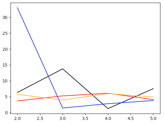
Our clumsy human operator “samples” at deterministic times $t_n = 2\pi n/\omega’$, where $\omega’ \ll \omega$ and the frequencies are incommensurable, i.e. their ratio is irrational. For instance, let’s take $\omega’ = \pi$ and $\omega = 10$. Then instead of randomising the initial conditions, we have a totally deterministic relation

We now plug this in to our dice and check the results are fair, once again using Pearson, but only for $\ell = 0.001, 0.01, 0.1$:

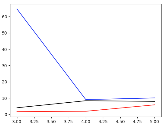
All three quickly approach a fair dice. We need to put the $\ell = 0.5$ dice on a separate plot, since it takes more than $10$ exploration times to arrive at something that looks fair:

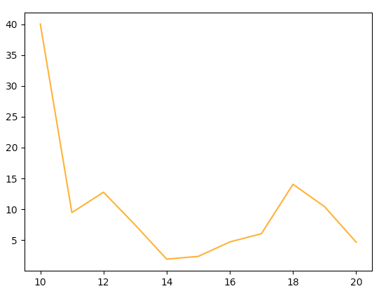
We can compute the number of exploration times it takes for the dice to become fair (as measured by the Pearson test) as a function of $\ell$. The relation is roughly linear:

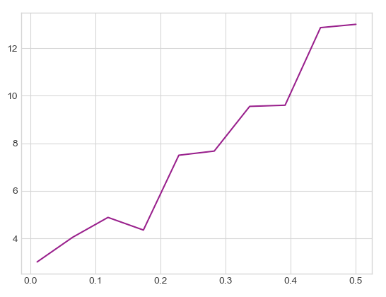
I’m not sure why this happens [⁷], but from this “onset-of-fairness” curve, we can select parameters to ensure our dice is statistically fair.

Conclusion

The randomness of a dice is not merely the consequence of symmetry, but rather, the combination of jitter and chaos. The dynamics amplify small jitters exponentially, so that even after a short dice roll, they thread through configuration space approximately uniformly. The jitter of initial conditions may be genuinely random, but can also arise deterministically from, e.g., two cycles which are out of sync. This leads to a simple, deterministic model of a dice roll, $X$:

where the parameters $\ell, \omega, k$ are chosen to ensure the dice is statistically fair. For instance, we can generate effectively random dice rolls with the following code:

import numpy as np

def dice_roll(n):
	f_n = (0.01/2)*(1 + np.sin(10*n))
	x = f_n*2**22 % 1
	return int(6*x) + 1

It’s difficult to rigorously show that dice exhibit chaotic dynamics. But hopefully our proofs-of-concept suggest that in deterministic games of chance, you really are dicing with chaos.

Appendix: code

I will get round to putting this in a repo at some point, but in the mean time, here is how to make all the plots. First up, here is our code for making the plot for a chaotic coin:

import matplotlib.pyplot as plt
import numpy as np

plt.style.use('seaborn-whitegrid')

def coin(ell, steps, numrolls = 100000): # simulate many coin flips
    tails = 0
    for i in range(numrolls):
        rand = np.random.uniform(0, ell) # uniformly select an initial condition
        evol = rand*(2**steps) % 1 # evolve chaotically
        if evol >= 0.5: # check whether heads or tails
            tails += 1
    return tails/numrolls

def explore(ell, lmbda = np.log(2)): # compute exploration timescale
    return np.log(1/ell)/lmbda
    
def coin_data(ell, multiples = 10, numrolls = 100000): # generate data for plotting
    timescale = np.ceil(explore(ell)) # makes timescale an integer
    data = []
    for n in range(1, multiples+1):
        bias = coin(ell, n*timescale, numrolls = 100000) # evolve for n timescales and compute bias
        data.append(bias) # add bias to data
    return data

data = coin_data(0.1, 10)
plt.plot(range(1, len(data)+1), data);
plt.show()
plt.clf()

data1 = coin_data(0.001, 6)
data2 = coin_data(0.01, 6)
data3 = coin_data(0.1, 6)
data4 = coin_data(0.5, 6)
plt.plot(range(1, len(data1)+1), data1, color='black');
plt.plot(range(1, len(data2)+1), data2, color='red');
plt.plot(range(1, len(data3)+1), data3, color='blue');
plt.plot(range(1, len(data4)+1), data4, color='orange');
plt.show()

Now for our chaotic dice with random jitter:

def dice_bias(ell, steps, sides = 6, numrolls = 100000): # simulate many dice rolls
    outcomes = [0] * sides
    pearson = 0
    for i in range(numrolls):
        rand = np.random.uniform(0, ell) # uniformly select an initial condition
        evol = rand*(2**steps) % 1 # evolve chaotically
        outcome = int(sides*evol) # calculate outcome
        outcomes[outcome] += 1
    for k in range(sides):
        pearson += numrolls*sides*(outcomes[k]/numrolls - 1/sides)**2 # compute pearson test statistic
    return pearson

def dice_data(ell, start_mult = 1, end_mult = 10, sides = 6, numrolls = 100000): # generate data for plotting
    timescale = np.ceil(explore(ell)) # makes timescale an integer
    data = []
    for n in range(start_mult, end_mult + 1):
        bias = dice_bias(ell, n*timescale, sides, numrolls = 100000) # evolve for n timescales and compute bias
        data.append(bias) # add bias to data
    return data

data5 = dice_data(0.001, 2, 5)
data6 = dice_data(0.01, 2, 5)
data7 = dice_data(0.1, 2, 5)
data8 = dice_data(0.5, 2, 5)
plt.plot(range(2, 6), data5, color='black');
plt.plot(range(2, 6), data6, color='red');
plt.plot(range(2, 6), data7, color='blue');
plt.plot(range(2, 6), data8, color='orange');
plt.show()

Here are chaotic dice with deterministic jitter:

def det_bias(ell, steps, sides = 6, numrolls = 100000): # simulate many dice rolls
    outcomes = [0] * sides
    pearson = 0
    for i in range(numrolls):
        init = (ell/2)*(1 + np.sin(10*i)) # deterministic jitter
        evol = init*(2**steps) % 1 # evolve chaotically
        outcome = int(sides*evol) # calculate outcome
        outcomes[outcome] += 1
    for k in range(sides):
        pearson += numrolls*sides*(outcomes[k]/numrolls - 1/sides)**2 # compute pearson test statistic
    return pearson

def det_data(ell, start_mult = 1, end_mult = 10, sides = 6, numrolls = 100000): # generate data for plotting
    timescale = np.ceil(explore(ell)) # makes timescale an integer
    data = []
    for n in range(start_mult, end_mult + 1):
        bias = det_bias(ell, n*timescale, sides, numrolls = 100000) # evolve for n timescales and compute bias
        data.append(bias) # add bias to data
    return data

dataA = det_data(0.001, 3, 5)
dataB = det_data(0.01, 3, 5)
dataC = det_data(0.1, 3, 5)
plt.plot(range(3, 6), dataA, color='black');
plt.plot(range(3, 6), dataB, color='red');
plt.plot(range(3, 6), dataC, color='blue');
plt.show()
plt.clf()

dataD = det_data(0.5, 10, 20)
plt.plot(range(10, 21), dataD, color='orange');
plt.show()

Finally, here is the code for measuring the onset of fairness:

def fair_time(ell, freq = 10, sides = 6, numrolls = 100000):
    pearson_check = 100 # initialise to be bigger than 10
    steps = 1
    while pearson_check > 10:
        outcomes = [0] * sides
        pearson = 0
        for i in range(numrolls):
            init = (ell/2)*(1 + np.sin(freq*i)) # deterministic jitter
            evol = init*(2**steps) % 1 # evolve chaotically
            outcome = int(sides*evol) # calculate outcome
            outcomes[outcome] += 1
        for k in range(sides):
            pearson += numrolls*sides*(outcomes[k]/numrolls - 1/sides)**2
        pearson_check = pearson
        steps += 1
    return steps/(explore(ell))

ells = np.linspace(0.01, 0.5, 10) # check ell between 0.01 and 0.5
fair_data = [fair_time(ell, numrolls = 10000) for ell in ells] # find onset of fairness
plt.plot(ells, fair_data, color='purple');
plt.show()