July 6, 2020. A derivative is a local linear approximation. Linear approximations are natural candidates for the function at “infinite zoom” since they are self-similar, i.e. fixed points of scaling. Here, I make the natural generalization to local approximation by an arbitrary self-similar curve. I also introduce random fractal approximations, and use these to motivate Brownian motion and more general Itô processes from an elementary perspective.

Straight line are fractals

A straight line is the simplest fractal, since if you pick any point on the line and zoom in, it looks the same. In other words, it is self-similar. Let’s check! A straight line passing through the origin has equation

\[y = L_m(x) = mx.\]

“Zooming in” is the same as rescaling the $x$ and $y$ axis by the same amount:

\[x \mapsto x' = \lambda x, \quad y\mapsto y' = \lambda y.\]

For any function $f$, rescaling both axes gives $y’ = f(x’)$, or

\[y = \lambda^{-1} f(\lambda x).\]

After this rescaling, most functions change, with $\lambda^{-1}f(\lambda x) \neq f(x)$. But a line does not change under this rescaling:

\[\lambda^{-1} L_m(\lambda x) = \lambda^{-1} (m (\lambda x)) = mx = L_m(x).\]

This is what we mean by self-similarity.

Derivatives are sometimes called local linear approximations. Let’s unpack that. If $f(x)$ is a real function, then its derivative at $x_0$ is defined as the limit of the slope of the secant line:

\[m = f'(x_0) = \lim_{h\to 0} \frac{f(x_0+h)-f(x_0)}{(x_0 + h)-x_0} = \lim_{h\to 0} \frac{\Delta f}{h},\]

if this limit exists. We can rewrite this as

\[f(x_0+h) - f(x_0) = L_m(h) + o(h),\]

where $o(h)$ stands for a function which shrinks faster than $h$ as $h \to 0$, $o(h)/h \to 0$. So, the “local” is in the fact that is a statement about behaviour in a neighbourhood of $x_0$, the “linear” is in the choice of function $L_m(h)$, and the “approximation” in $o(h)$.

Zooming in

What has this got to do with fractals? Linear approximations are natural since they are what you see at “infinite zoom”. More precisely, we can think of infinite zoom as producing fixed points of zooming. This is exactly what we mean by self-similarity, but it’s useful to explain in terms of the language of fixed points. A fixed point $\hat{x}$ of a function $g$ satisfies $g(\hat{x}) = \hat{x}$. Applying the function to the point $\hat{x}$ does nothing. We can define a zooming operation $Z_\lambda$, for $\lambda > 0$, which acts on real functions as follows:

\[Z_\lambda [f] = \lambda^{-1} \circ f \circ \lambda, \quad Z_\lambda [f](x) = \lambda^{-1}f(\lambda x).\]

Here, we’ve overloaded $\lambda$ by making it stand for both a number and the function which multiplies by $\lambda$, but hopefully that’s not confusing. A self-similar function $F$ is a fixed point of $Z_\lambda$, in the sense that

\[Z_\lambda[F] = F, \quad Z_\lambda [F](x) = \lambda^{-1}F(\lambda x) = F(x),\]

just like straight lines as we calculated above.

When we do a local linear approximation, we are zooming in until the curve is approximately self-similar, at least when we centre the coordinates at $x = x_0$ and $y = f(x_0)$. In this case,

\[\Delta f = f(x_0 + h) - f(x_0) \mapsto \Delta f' = \lambda \Delta f, \quad h = (x_0 + h) - x_0 \mapsto h' = \lambda h,\]

while our local linear approximation changes as

\[\Delta f = L_m(h) + o(h) \mapsto \lambda^{-1} \left[ L_m(\lambda h) + o( \lambda h)\right] = L_m(h) + \lambda^{-1}o( \lambda h).\]

It’s not hard to see that the last term is also $o(h)$, since

\[\lim_{h\to 0} \frac{o( \lambda h)}{\lambda h} = \lim_{h'\to 0} \frac{o(h')}{h'} = 0.\]

So, local linear approximation could also be thought of as local approximation by a self-similar function. This is naturally associated to the function at “infinite zoom”, since self-similar functions are fixed points of scaling.

Fractal approximation

Local linear approximation is a natural thing to do because lines look the same when you zoom in. But they are not the only functions with this property! We could replace a line with any self-similar function. It is therefore natural to consider local approximation by a self-similar fractal $F$, when

\[\Delta f = F(h) + o(h).\]

This is unique up to terms which vanish as $o(h)$, simply because

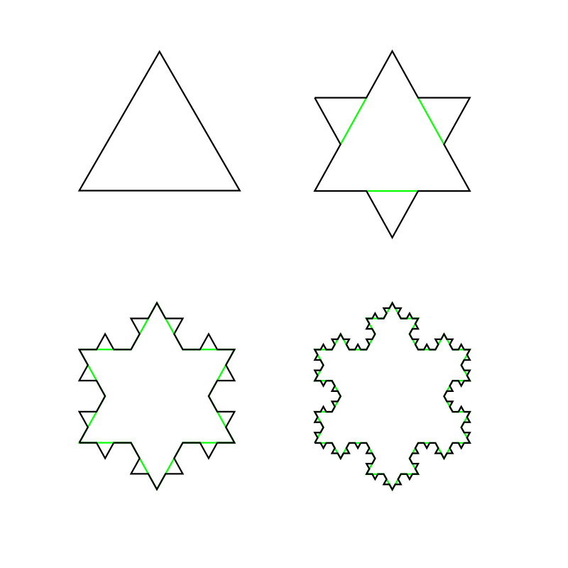
\[\Delta f = F(h) + o(h) = G(h) + o(h) \quad \Longrightarrow \quad F(h) - G(h)= o(h).\]

As a trivial example, a self-similar function $F(x)$ is locally approximated by $F(x)$. So the Koch curve, made by iteratively adding snowflake-like stellae, is locally approximated by a Koch curve! To get an interesting local approximation, we can deform the star at large scales, but leave it alone (or deform in some $o(h)$ way) as we zoom in.

Here, we obviously have a curve rather than a function per se, but the same idea holds.

You may have noticed that I left $\lambda$ ambiguous when defining self-similarity. Is a function $F$ self-similar if $Z_\lambda[F] = F$ for any $\lambda> 0$, or just a certain fixed $\lambda$? The straight line has the distinction of looking the same at any scale, so $Z_\lambda[L_m] = L_m$ for any $\lambda$. In fact, a straight line is the only “nice” curve with this property. For instance, if we assume that our self-similar curve itself has a (normal linear) derivative at some point $x$, then

\[F'(x) = \lambda^{-1} \frac{d}{dx}F(\lambda x) = F'(\lambda x).\]

If this is true for any $\lambda$, the slope at any two points is the same, and we get a straight line. Note that we only need a derivative at one point to get a straight line from self-similarity under arbitrary zooms. This shows that if there are other curves with this property, they are nowhere differentiable.

The same but different*

What if zoomed in differently on the $x$ and $y$ axes? In other words, let’s consider a generalization of the $Z_\lambda$ operator, $Z_{(\alpha,\beta)}$, which is defined by

\[Z_{(\alpha,\beta)}[f] = \alpha^{-1} \circ f \circ \beta,\]

which obeys $Z_{(\lambda,\lambda)} = Z_\lambda$. This can also have fixed points, $Z_{\alpha, \beta}[F] = F$, fractals which scale differently in different directions. As an example, polynomials are fractals in this sense. For instance, consider $F(x) = \sqrt{x}$. Then

\[Z_{(\alpha,\beta)}[F] = \alpha^{-1} \sqrt{\beta x} = \alpha^{-1}\sqrt{\beta} f(x),\]

and hence $F$ is a fixed point of $Z_{(\alpha, \alpha^2)}$ for any $\alpha$. And indeed, we can also make local approximations in terms of these inhomogeneously self-similiar curves.

The last ingredient in this pot-pourri of ideas is randomness. Instead of a fixed, deterministic function $f$, I can imagine some function $\hat{f}$ which fluctuates randomly. It could be stock market data, a casino’s holdings, or the position of a bacterium motoring around in search of nutrients. Whatever the source of randomness, it may make the function jumpy enough to be non-differentiable, i.e. jagged when you zoom in, but not describable by a deterministic fractal either. But perhaps it can be described by a random fractal!

First, let’s see what a local random approximation means (also called stochastic derivatives). A natural guess is

\[\hat{f}(x_0 + h) - \hat{f}(x_0) = \Delta \hat{f}(h) \sim \mathcal{P}(h) + o(h),\]

where $\sim$ indicates that $\Delta \hat{f}$ is distributed according to some probability distribution $\mathcal{P}(h)$, depending on $h$ and possiby the value at $\hat{f}(x_0)$. We will use random fractal as a clickbait term for “self-similar probability distribution”, i.e. such that $\mathcal{P}(h)$ is a fixed-point of some $Z_{(\alpha,\beta).}$ More precisely, we mean that

\[\alpha^{-1}\Delta \hat{f} \sim \mathcal{P}(\beta h) + o(h).\]

To see what sorts of probability distributions are reasonable, first, note that we can split up a step of size $h$ into two steps, say $k$ and $h - k$. Then

\[\Delta \hat{f}(h) = \Delta \hat{f}(k) + \Delta \hat{f}(h-k)\]

suggests the distribution must satisfy

\[\mathcal{P}(k) + \mathcal{P}(h-k) \sim \mathcal{P}(h) + o(h).\]

This additivity property is somewhat rare among probability distributions. But we have already encountered it above: for a straight line! More precisely, ordinary derivatives—local linear approximations—have the nice property that

\[\Delta F(k) + \Delta F(h-k) = mk + m(k-h) + o(h) = mh + o(h) = \Delta F(h).\]

We will call this the additivity constraint.

Brownian motion*

We’ll look at a simple example: the normal distribution $\mathcal{N}(\mu, \sigma^2)$ of mean $\mu$ and variance $\sigma^2$. This has the neat property that a sum of independent normals is normal, with

\[\mathcal{N}(\mu_1, \sigma_1^2)+\mathcal{N}(\mu_2, \sigma_2^2) \sim \mathcal{N}(\mu_1 +\mu_2, \sigma_1^2+\sigma_2^2).\]

It’s clear, then, that we can satisfy our additivity constraint by setting $\mathcal{P}(h) = \mathcal{N}(0, h)$. We have just constructed Brownian motion! More precisely, we say that $\hat{F}$ is undergoing Brownian motion if

\[\Delta \hat{F}(h) \sim \mathcal{N}(0, h) + o(h).\]

In fact, we can set some initial position $\hat{F}(x_0)$, and then define the rest of the random function $\hat{F}$ by letting it wander Brownianly, i.e. by making random normal steps. This makes it the sort of continuum limit of a discrete random walk.

Although Brownian motion is not self-similar in the homogeneous sense we introduced earlier, it is inhomogenously self-similar. Rescaling the vertical distance by some factor rescales the variance by that factor squared (since variance is spread squared), so that

\[\alpha^{-1}\Delta \hat{F}(h) \sim \mathcal{N}(0, \alpha^{-2} h) + o(h).\]

Clearly, we can offset this by rescaling $h$ by $\alpha^2$, so that Brownian motion is indeed a random fractal, a fixed point of $Z_{(\alpha, \alpha^2)}$ for any $\alpha$. Put differently, Brownian motion is the random fractal cousin of the square root! In fact, it’s clear that we can scale Brownian motion and additivity will still work:

\[\Delta \hat{F}(h) \sim \mathcal{N}(0, \sigma^2 h) + o(h) = \sigma\mathcal{N}(0, h) + o(h).\]

In Leibniz notation, we take the limit of very small $h$, and replace $\Delta$ with $d$. We then write Brownian motion as

\[d\hat{F} = \sigma \, dW,\]

where $W$ stands for Wiener process, after Norbert Wiener, who first defined it. But really, this is shorthand for the notation with $h$ above.

The final Itôration**

In this last section, we are going to forget about self-similarity, and focus on the additivity property. We have seen two local approximations that possess it so far: ordinary linear approximations and the Wiener process, or Brownian motion. If we add these two together, they will maintain the additivity property! Thus, we are led to consider the somewhat odd-looking local approximation

\[\Delta \hat{F} = m h + \sigma \mathcal{N}(0, h) + o(h),\]

or in Leibniz notation,

\[d\hat{F} = m \,dx + \sigma \, dW.\]

This is called Brownian motion with drift, since in addition to the random Gaussian step with zero mean, there is a (locally) linear drift $mh$. It’s easy to verify this is additive, since

\[\begin{align*} \Delta \hat{F}(k) + \Delta \hat{F}(h-k) & = m [k + (h-k)] + \sigma \mathcal{N}(0, k) + \sigma \mathcal{N}(0, h - k) + o(h) \\ & \sim \Delta \hat{F}(h). \end{align*}\]

Technically, Brownian drift is for fixed $m$, but we can also imagine the gradient changing with $x_0$, the position we’re doing the approximation near. In fact, let’s just call it $x$, since this won’t result in ambiguity, and write

\[d\hat{F} = m(x) \,dx + \sigma \, dW.\]

While we’re at it, we may as well make the random steps change with $x$:

\[d\hat{F} = m(x) \,dx + \sigma(x) \, dW.\]

And for that matter, we could even make them depend on the current value of the function, $y = \hat{F}(x_0)$. That gives us a very general looking way to update our random function:

\[d\hat{F} = m(x, y) \,dx + \sigma(x, y) \, dW.\]

Locally, we just have a straight line plus Brownian motion. But the parameters can change depending on where we are on the $(x, y)$ plane. This is called an Itô process, after Japanese mathematician Kiyosi Itô. This sounds like a useless generalization, but we will give two specific and useful examples. First, if $m(x, y) = -my$ for a constant $y$, then we have the Ornstein–Uhlenbeck process:

\[d\hat{F} = -m y \,dx + \sigma \, dW.\]

This walks randomly, but rather than drift with fixed $m$, the larger the value of the function, the greater the strength of the drift back to $y = 0$ (if $m$ is positive) or away (if $m$ is negative). This describes a hot spring, for instance, trying to relax back to its equilibrium length while that length also jitters due to random thermal motion.

Our second example is the Black–Scholes-Merton process, which is like Ornstein-Uhlenbeck, but now the size of random steps also depends on $y$:

\[d\hat{F} = r y \,dx + \sigma y \, dW.\]

In this case, $\hat{F}$ models stock prices! Here, $r$ is a compound interest rate. For continuous compounding, the value of the stock after a short time ($rt \ll 1$) is

\[y' = y e^{rt} \approx y(1 + rt) \quad \Longrightarrow \quad dy = y' - y = ry t.\]

This gives the result above when the short time is $t = dx$. The stock value will also fluctuate randomly by an amount $\sigma\, dW$, assuming the variance $\sigma^2$ of market fluctuations is constant in time. Since this is per dollar, the total fluctuation in value is $\sigma y\, dW$. This leads to an equation for the value of options — the option of buying or selling stocks at some later date — called the Black–Scholes-Merton equation, and which won Scholes and Merton the Nobel prize in economics in 1997. So, although we started with straight lines, the path becomes somewhat more jagged, leading us to fractals, forces and finance!