Contents
1. Introduction
Prerequisites: basic quantum mechanics, linear algebra, and some background in quantum computing.
In quantum mechanics, a system is described by a vector in a Hilbert space. Hilbert space is very, very large, which is one of the reasons quantum computers are more powerful than classical ones. But this leads to two problems: how can we effectively use a big Hilbert space? And how can we picture what’s going on? It turns out that, sometimes, the answers coincide. In this tutorial, we will see that, in seeking a convenient way to visualize high-dimensional Hilbert spaces, we will naturally arrive at the quantum Fourier transform (QFT), a workhorse protocol which is dramatically faster on a quantum computer than its classical counterpart.
2. Polygons
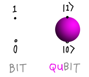
To make our problem sharper, let’s consider the problem of visualizing the simplest nontrivial system, a single qubit. The classical bit can be in states $b = 0, 1$. Each of these is promoted to a basis state of the qubit, $|b\rangle$. A general vector in this Hilbert space is
\[|\psi\rangle = \alpha |0\rangle + \beta |1\rangle, \quad \alpha, \beta \in \mathbb{C}.\]Without further work, the space of states lives in $\mathbb{C}^2 \simeq \mathbb{R}^4$, which is already impossible to picture. Our visual cortex evolved for three dimensions only! Luckily, the global phase ambiguity and normalization constraint mean we can directly draw the space of single qubit states on a sphere, as below:
But any bigger, and the method fails! So trying to directly visualize things does not scale at all. The question becomes: is there useful indirect way to picture points in an arbitrary Hilbert space, and help us navigate the hugeness?
2.1. Form and function
The answer is a resounding yes, and in fact, you probably (secretly) already know the solution. Consider a graph $y = f(x)$ on the Cartesian plane. You can add functions together and multiply them by real numbers, and this turns the set of functions into a vector space! Moreover, it’s an infinite-dimensional vector space, since (loosely speaking) we can think of each point $x$ as a basis vector.
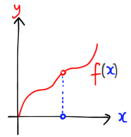
We certainly don’t need all of those dimensions! Instead of a continuous variable $x$, we can imagine a finite number of points labelled by $k \in \{0, 1, \ldots, d- 1\} =: [d]$. Then we can represent a vector in $\mathbb{R}^d$ as a map $f: [d] \to \mathbb{R}$. We can add and multiply these maps as usual, $f +g, \lambda f$. To figure out which $k \in [d]$ is responsible for which point on the plane, we simply project onto the $x$ axis.
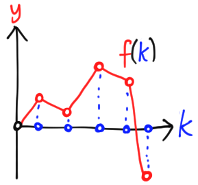
What about a complex vector with $d$ components? A hack is simply to treat $\mathbb{C}^d \simeq \mathbb{R}^{2d}$, but then multiplying a vector a complex number looks very unnatural. Instead, we once again take inspiration from a familiar infinite-dimensional trick: drawing the image of a parametrized curve $f: [d] \to \mathbb{C}$, where $I \subseteq \mathbb{R}$. We lose the information about which element of $[d]$ is associated with a point on the curve, as the image below shows.
Of course, we could stack copies of $\mathbb{C}$ on top of each other, but this is harder to draw. More importantly, it is unnecessary in finite dimensions! We can recover the information about which $k$ maps to which complex number as long as the function is into, i.e. there are no overlaps. We simply draw a chain of points, and mark the first some way, e.g. with a black dot.
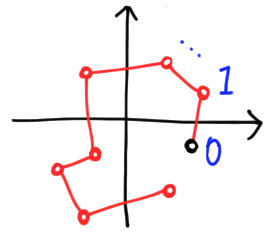
There is a loose end here—or rather, two loose ends! The first and last point on the chain are unattached. If we connect them, the chain becomes a closed loop. There is no law against this, but it does make the correspondence between points and arguments ambiguous unless we specify a direction to go around the loop. We can do this by making edges directed:
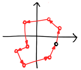
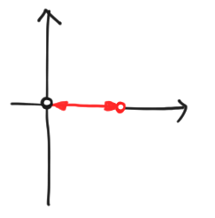
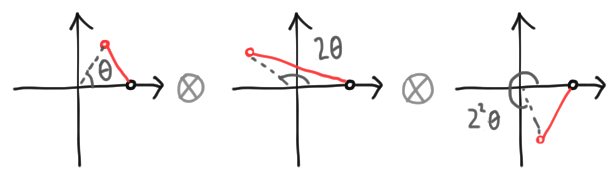
So rather than a chain with one marked end, vectors are now marked, directed polygons. This gives us a way to represent any vector in any finite-dimensional Hilbert space. These polygons add component-wise, and scalar multiply by complex numbers in a natural way. If we write an arbitrary scalar as $z = \lambda e^{i\theta}$, multiplication by $z$ scales the whole figure by $\lambda$ and rotates it an angle $\theta$ counterclockwise, both with respect to the origin. We give examples below:
All of this holds for open chains as well. But polygons are preferable for reasons we will discover shortly.
2.2. Battle of the bases
Let’s see what we can do with all this pictorial power at our disposal. A warm-up task is simply to draw the computational basis states, $|k\rangle$ for $k \in [d]$, since (as the name suggests) this is a good basis for doing computations. Unfortunately, our method fails at the first hurdle! Here’s what most of the basis vectors look like:
It starts at $0$, stays there for a while, goes to $1$ at the $k$th node, then returns to the origin. We can’t even tell what state we’re in unless we introduce more labels!
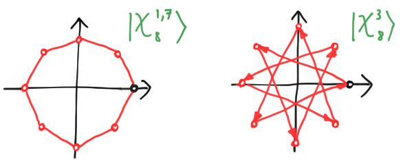
There are two ways we could see this: a failing of our method, or a failing of the basis. We will, of course, take the partisan viewpoint that the basis is at fault, and look for a better one. If we were dealing with chains, the way forward would be decidedly ugly and non-unique. But our choice of polygons pays off, since the uniquely nice objects to use are the regular polygons! These consist of points equally spaced around the circle, or
\[\vec{v} = \sum_k r e^{ik\theta} |k\rangle,\]for some constant $r$ and angle $\theta$. To ensure we end up back where we started after $d$ points, we require $d\theta$ to be a multiple of $2\pi$, or $\theta = 2\pi s/d$ for some integer $s$. The $r$ is irrelevant for choosing a basis, so we set it to $1$, and normalize to get states. We define the resulting regular polygonal vectors and eigenstates by
\[\vec{\chi}^s_d := \sum_{k=0}^{d-1} e^{2\pi i s/d} |k\rangle, \quad |\chi^s_d\rangle := \frac{1}{\sqrt{d}}\vec{\chi}^s_d. \label{chivec} \tag{1}\]We can directly check that these not only form a basis, but that the eigenstates are orthonormal. Assuming $t \neq s$ (modulo $d$), we have
\[\begin{align*} \langle \chi^{t}_d |\chi^s_t\rangle & = \frac{1}{d}\sum_{k=0}^{d-1} e^{2\pi i (s-t)/d} = \frac{1}{d} \cdot \frac{1 - e^{2\pi i d (s-t)/d}}{1 - e^{2\pi i (s-t)/d}} = 0, \end{align*}\]where we summed using a geometric series, and observe that the numerator vanishes when $s - t$ is an integer. Thus, the $|\chi^s_d\rangle$ form an orthonormal basis. We give a slightly more elegant (optional) motivation from group theory below.
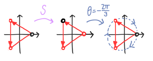
Group theory easter egg. Our choice of representation is guided by the structure we put on the set $[d]$ itself. When we draw vectors as marked chains, we are effectively thinking of $[d]$ as an ordered set. When we draw it as a polygon, we are implicitly thinking of $[d]$ as a cyclic group, say $[d] = \mathbb{Z}/d\mathbb{Z}$. This group is generated by the operation of subtracting $1$, or $S: |k\rangle \mapsto |k-1\rangle$ modulo $d$. This corresponds to a unitary matrix
\[S = \left[ \begin{matrix} 0 & 0 & 0 & \cdots & 0 & 1 \\ 1 & 0 & 0 & \cdots & 0 & 0\\ 0 & 1 & 0 & \cdots & 0 & 0\\ &&&\ddots& \\ 0 & 0 & 0 & \cdots & 1 & 0 \end{matrix} \right].\]We will choose our basis to be eigenstates of $S$. The first thing to note is that $S^d = \mathbb{I}$, since after $d$ shifts we end up where we started. For any eigenstate $|\psi\rangle$ with eigenvalue $\omega$, it follows that
\[S^d |\psi\rangle = \omega^d |\psi\rangle = |\psi\rangle,\]and hence $\omega^d = 1$. Thus, $\omega$ must be a root of unity, and $|\psi\rangle$ is mapped to itself up to a global phase. For a polygon, $S$ shifts the black dot along a polygon. If $|\psi\rangle$ is an eigenstate, we can undo this by a rotation, which means precisely that $|\psi\rangle$ is regular! We illustrate for an equilateral triangle below:
Let’s now find the eigenstate of $S$ associated with a $d$th root of unity $\omega$. Writing $|\psi\rangle = \sum_k \alpha_k |k\rangle$, we have
\[(S - \omega) |\psi\rangle = \sum_k (\alpha_k |k-1\rangle - \omega\alpha_k |k\rangle) = \sum_k (\alpha_{k+1} - \omega \alpha_k)|k\rangle = 0,\]where we relabelled the dummy index $k \to k +1$ in the first term. This means we have a relation $\alpha_{k+1} = \omega\alpha_{k}$ for all $k$, modulo $d$. Without loss of generality (and ignoring normalization for the moment), we can set $\alpha_0 = 1$ and iterate, so that $\alpha_k = \omega^k$. If we choose a primitive root of unity $\omega_d = e^{2\pi i/d}$, then all roots of unity have the form $\omega_d^{s}$ for some $s \in [d]$. This gives rise to the $d$ unnormalized eigenvectors, and corresponding eigenstates, we found in (\ref{chivec}):
\[\vec{\chi}^s_d := \sum_{k=0}^{d-1} e^{2\pi i s/d} |k\rangle, \quad |\chi^d_s\rangle := \frac{1}{\sqrt{d}}\vec{\chi}^s_d.\]These automatically form a basis, and in fact are orthogonal, since they are eigenstates of a unitary operator.
2.3. That’s a wrap!
When picturing these regular polygons, there are a few peculiarities to keep in mind. First, when $s = 0$, all the points lie at $1$. This is a sort of degenerate regular polygon where, between each node, we execute a full revolution around the origin:
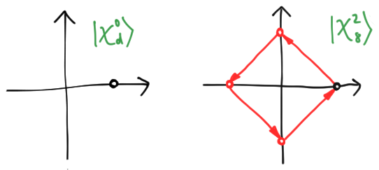
There is a less extreme degeneracy where regular polygons overlap themselves. We give the example of $d = 8, s = 2$ above, where a “regular octagon” has degenerated into two squares sitting on top of each other. But although points can degenerate into each other, the basis elements are always distinct, provided you know $d$: you simply see where the first arrow goes. If it arrives at a point $e^{i\theta}$, then $s = d\theta/2\pi$. Thus, we have indeed eliminated the ambiguity that plagued the computational basis, without any need for additional labels.
Let’s give a simple example. For a qubit, $d = 2$, and the two polygonal states are
\[\begin{align*} |\chi^0_2\rangle & = \frac{1}{\sqrt{2}}\sum_{k=0}^1 e^{2\pi i 0 \cdot k/d}|k\rangle = \frac{1}{\sqrt{2}}(|0\rangle + |1\rangle) = |+\rangle \\ |\chi^1_2\rangle & = \frac{1}{\sqrt{2}}\sum_{k=0}^1 e^{2\pi i 1 \cdot k/d}|k\rangle = \frac{1}{\sqrt{2}}(|0\rangle - |1\rangle) = |-\rangle. \end{align*}\]These are just the familiar eigenstates $|\pm\rangle$ of the $X$ observable! We draw them below:

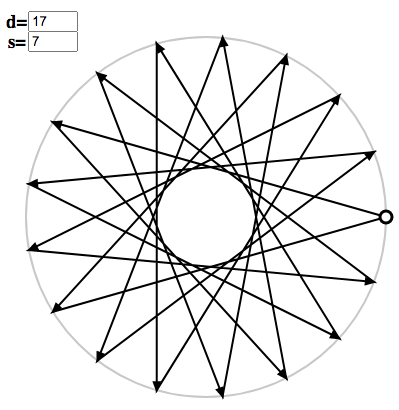
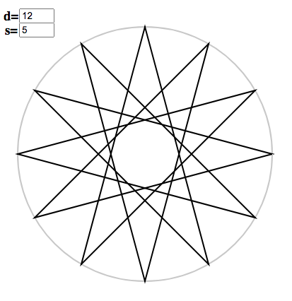
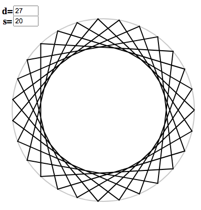
You can generate polygons for arbitrary $s$ and $d$ using the polygon applet. For instance, we can enter $d = 17$ and $s = 7$, and the corresponding basis element will be displayed:
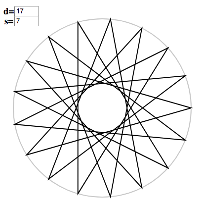
You can toggle arrow tips with “t”:
The wrapped polygons obey a simple pattern. For any $d$, there are only two convex, non-degenerate regular polygons, i.e. regular $d$-gons, occurring at $s = 1$ and $s = d-1$. For other values of $s$ which are relatively prime with $d$, we get stellated non-degenerate polygons, which have $d$ sides but intersecting edges.
To understand the general case, note that if $f$ is a common divisor of $d$ and $s$ (written $f | d$, $f | s$), then $k = d/f$ is an integer such that
\[\frac{2\pi ks}{d} = \frac{2\pi ds}{df} = \frac{2\pi s}{f} \in 2\pi \mathbb{Z}.\]Thus, at the $k$th node the polygon wraps back to $1$. If $g = \text{gcd}(s, d)$ is the greatest common divisor, then $k = d/g$ is the first node at which the polygon $\vec{\chi}^s_d$ returns to $1$. Hence, $\vec{\chi}^s_d$ is a polygon with $d/g$ sides which wraps itself $g$ times. This has an amusing (and optionally readable) consequence for number theory.
Number theory easter egg. The count of $s \in [d]$ relatively prime to $d$ is given by Euler’s totient function $\phi(d)$. Similarly, $\phi(d/f)$ counts the values $s$ for which $\text{gcd}(d, s) = f$, since
\[\text{gcd}(d, s) = f \quad \Leftrightarrow \quad \text{gcd}(d/f, s) = 1.\]Thus, $\phi(d/f)$ counts the regular polygons wrapping $f$ times. Since $d/f = f’$ is just another way of enumerating factors of $d$, and every polygon must wrap $f$ times for some factor $f$, we deduce that
\[\sum_{f|d} \phi(f) = d.\]This identity was first proved by Gauss in his Disquisitiones Arithmeticae.
3. The Quantum Fourier Transform
The purpose of the last section was to find a way to draw vectors in big Hilbert spaces. The computational basis is ill-adapted to this representation, so we came up with a new basis which jived better. But we shouldn’t throw out the computational basis with the bath water! It’s the closest thing we have to working with bit strings, and hence a natural place to do many quantum information-processing tasks.
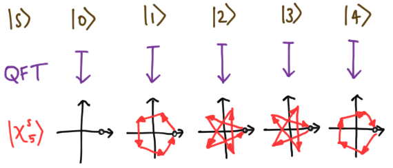
We can have our basis and eat it too if we find a way to convert between the computational and polygonal vectors. This is where the Quantum Fourier Transform (QFT) comes from. It is simply the active change of basis from computational states to regular-polygonal states,
\[\text{QFT}_d: |s\rangle \mapsto |\chi^s_d\rangle, \label{qftd} \tag{2}\]extended linearly to the full Hilbert space. As a simple example, our $d =2$ example above shows that $\text{QFT}_2 = H$, the Hadamard matrix. We show the action on the basis for $d = 5$ below:
In general, it is a matrix (also called the Walsh-Hadamard matrix) with elements
\[\langle j|\text{QFT}_d |k\rangle = \langle j|\chi^k_d\rangle = \frac{1}{\sqrt{d}}\omega_d^{jk}.\]We could finish the tutorial here if we liked, but in the next few sections, we’ll outline some fun features of the QFT, including a neat geometrical interpretation of the Fourier coefficients, the advantages of factorization, and algorithmic aspects.
3.1. Getting unhinged
The QFT is, by definition, an active change of basis. In the context of linear algebra, it’s slightly more natural to think of a passive change of basis, which finds the coefficients $A_s$ in the polygonal basis,
\[|\psi\rangle = \sum_k \alpha_k |k\rangle =: \sum_s A_s |\chi^s_d\rangle.\]Since $|\chi^s_d\rangle$ is an orthonormal basis, it’s easy to extract $A_s$ from an overlap:
\[\begin{align*} A_s = \langle \chi^s_d |\psi\rangle & = \sum_k \alpha_k \langle \chi^s_d|k\rangle = \frac{1}{\sqrt{d}}\sum_k \alpha_k \omega_d^{-ks}. \end{align*} \label{a_s} \tag{3}\]This passive operation is called the Discrete Fourier Transform (DFT). The DFT and QFT are just inverses of each other, in the sense that the coefficients of a quantum Fourier-transformed vector, in the computational basis, are given by the DFT:
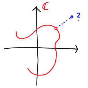
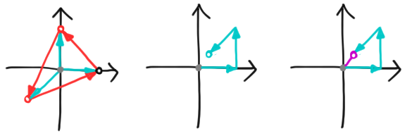
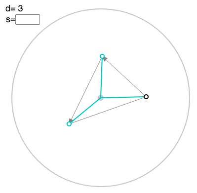
\[\text{QFT}|\psi\rangle = \sum_k \alpha_k \text{QFT}|k\rangle = \frac{1}{\sqrt{d}}\sum_s \sum_k \alpha_k \omega_d^{ks} |s\rangle = \sum_s A_{-s}|s\rangle.\]It turns out that the coefficients (\ref{a_s}) have a simple geometric interpretation. We can take a vector $\vec{v} = \sum_k v_k |k\rangle$, and concatenate the complex numbers $v_k$, tip-to-tail, on the complex plane. We’ll call this a linkage. The value $V(\vec{v})$ is the point at which the last arrow of the linkage ends. We give an example for a qutrit below, with the usual polygon in red, the linkage in cyan, and the value in purple:
The overlap $(\vec{\chi}^s_d)^\dagger \vec{v}$ is just the value of the vector
\[\vec{v}_s = \sum_k v_k \omega_d^{-ks} |k\rangle.\]Mechanically, we can think of $\vec{v}_s$ as a hinged motion of the linkage associated with $\vec{v}$. We leave the first arrow in the linkage alone, then rotate the rest by $\omega_d^{-s}$. Then we move along and rotate all but the first two by $\omega_d^{-s}$. We continue in this way until $v_k$ has been rotated by $\omega_d^{-ks}$. Finally, to get the overlap with $|\chi^s_d\rangle$, we simply divide by $\sqrt{d}$.
You can gain intuition for how the Fourier transform is related to hinged motion in this linkage applet. Click to create the points in the vector, which are now displayed as complex numbers, i.e. arrows from the origin:
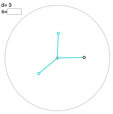
You can toggle a faint polygon with “p”:
To see the corresponding linkage, press “l”:
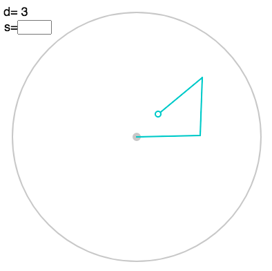
You can also display the value using “v”:
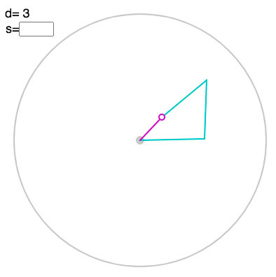
Finally, you can enter the parameter $s$ for the Fourier transform in the box above left:
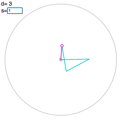
In fact, you can enter arbitrary $s$ to see a “continuous” hinged motion, though the QFT only involves integer $s$. We will use $x$ to denote the arbitrary argument, and let $s$ always stand for integers. The Fourier coefficient $A_{-s}$ is divided by a factor of $\sqrt{d}$, but we have omitted this for visual clarity.
3.2. Divide and conquer
It turns out that the QFT and the DFT are tremendously important operations in their own right. For instance, if we take the limit of a continuous curve on the complex plane, with $d \to \infty$, we recover Fourier series. We will focus our efforts in a different direction, however. A quantum computer is a large quantum system, with Hilbert space of size $d$ built out of $n$ smaller quantum systems of size $d_i$. The Hilbert spaces are related by the tensor product:
\[\mathcal{H}_{d} \simeq \mathcal{H}_{d_0} \otimes \mathcal{H}_{d_1} \otimes \cdots \otimes \mathcal{H}_{d_{n - 1}},\]where $d = d_0 d_1 \cdots d_{n - 1}$, and $\simeq$ indicates that these spaces are isomorphic, but in a way we have to specify. As a special but important case, a quantum computer made from $n$ qubits, with $d_i = 2$, has a Hilbert space of dimension $2^n$. Interesting things happen for the QFT when the Hilbert space factorizes. Consider the simple case $d = ab$, with
\[\mathcal{H}_d \simeq \mathcal{H}_a \otimes \mathcal{H}_b.\]In order to canonically identify states on the left and right, we define
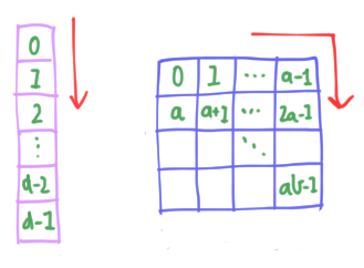
\[|k(m, n)\rangle = |na + m\rangle \simeq |m\rangle \otimes |n\rangle \label{kmn} \tag{4}\]for $m \in [a], n \in [b]$. It’s easier to see what’s going on using a picture. Without factorization, we imagine the indices $s \in [d]$ arranged in a single column of length $d$, and read downwards. When we factorize, we rearrange this column into a $b \times a$ grid or index matrix, and read like English, left-to-right and down:
Let’s see what this implies for the QFT. For a regular polygon $\vec{\chi}^s_d$, the coefficient of $|k\rangle$ given by (\ref{kmn}) is
\[e^{2\pi i ks/d} = e^{2\pi i (na + m)s/ab} = e^{2\pi i ms/ab}e^{2\pi i ns/b} = \omega_a^{sm/b}\omega_b^{sn}. \label{prod} \tag{5}\]In the tensor product basis,
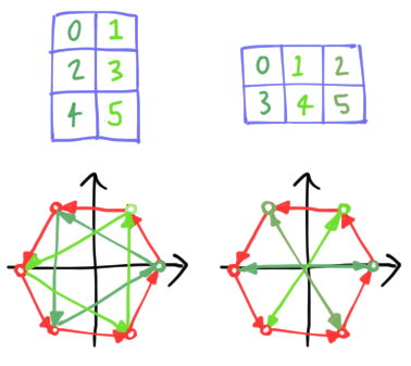
\[\vec{\chi}^s_d \simeq \sum_{mn} \omega_a^{sm/b}\omega_b^{sn}|m\rangle\otimes|n\rangle = \sum_{m}\omega_a^{sm/b}|m\rangle \otimes \sum_n \omega_b^{sn} |n\rangle = \vec{\chi}^{s/b}_a \otimes \vec{\chi}^s_b.\]Here, $\vec{\chi}^s_b$ is a regular polygonal basis element, but $\vec{\chi}^{s/b}_a$ is an odd beast. Despite the notation, it is not a regular polygon at all, but rather serves to make copies of $\vec{\chi}^s_b$, offset by angles $\theta = 2\pi s/d$. For this reason, we call it a copygon. As a simple example, we can factorize a regular hexagon $\vec{\chi}^1_6$ in two ways, as two triangles or three digons:
\[\vec{\chi}^1_6 \simeq \vec{\chi}^{1/3}_2 \otimes \vec{\chi}^{1}_3 \simeq \vec{\chi}^{1/2}_3 \otimes \vec{\chi}^{1}_3.\]We picture the decompositions into copies of the second factor below:
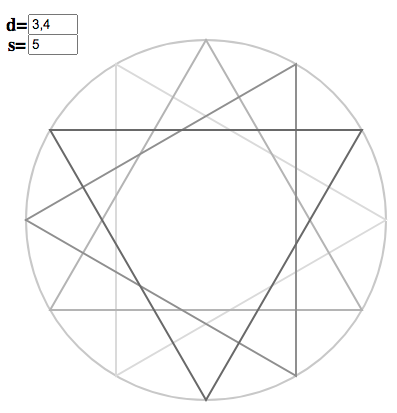
The coloured node indicates the first node of the copy. Once more, you can play with your own examples and build up intuition using the polygon applet. Suppose you are interested in $d = 12, s = 5$. Without factorizing, it looks like:
To exploit $12 = 3 \times 4$, in the applet, replace $12$ by $3, 4$:
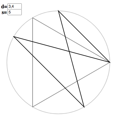
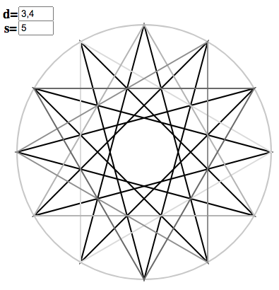
The dark figure is the copygon $x = 5/3, d= 4$, while the grey triangle is the regular polygon $x = 5, d = 3$. Pressing “c” will perform the copying:
The triangles are arrayed around the circle, according to the instructions of the copygon. In the index matrix, triangles correspond to columns and copygon entries to rows, so we read “across” triangles to generate $\vec{\chi}^5_{12}$. We can demonstrate the correspondence (without recourse to a matrix) by toggling “f” for “full polygon”:
In the general case $d = d_0 d_1\cdots d_{n-1}$, we can simply iterate this procedure:
\[\vec{\chi}^s_{d} \simeq \vec{\chi}^{sd_{n-1}/d}_{d_{n-1}} \otimes \cdots \otimes \vec{\chi}^{s/d_0}_{d_1} \otimes \vec{\chi}^{s}_{d_0}. \label{prods} \tag{6}\]This can be pictured using the polygon applet, for example, $s = 1$ and $d = 2 \times 3 \times 4$:
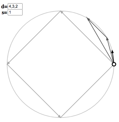
[Note the reversal of the order of factors. I intend to fix this!] We can view this as decomposing $d$ into a higher-dimensional index tensor, which iterates over the tensor product basis, but we won’t worry about the details.
3.3. Building up to the QFT
Crudely speaking, a quantum computer is a bunch of small, easily manipulable modules joined together in a useful way. Typically, the $n$ smaller systems have the same Hilbert space dimension, which we will take to be $d_i = a$. The quantum computer then has a Hilbert space of size $d = a^n$, and (\ref{prods}) becomes
\[|\chi^s_{d}\rangle \simeq |\chi^{sa^{1-n}}_{a}\rangle\otimes \cdots \otimes |\chi^{s/a}_{a}\rangle \otimes |\chi^{s}_{a}\rangle. \label{qft} \tag{7}\]This has a simple interpretation in our pictorial language. We build the initial (leftmost) copygon with $x = sa^{1-n}$, then expand $x$ by a factor of $a$ a total of $n-1$ times:
\[|\chi^{sa^{1-n}}_{a}\rangle \mapsto |\chi^{sa^{1-n} \cdot a}_{a}\rangle = |\chi^{sa^{2-n}}_{a}\rangle \mapsto |\chi^{sa^{2-n} \cdot a}_{a}\rangle = |\chi^{sa^{3-n}}_{a}\rangle \mapsto \cdots \mapsto |\chi^{s}_{a}\rangle.\]Of course, we need to tensor together all these intermediate results, so we start with $n$ copies of the initial copygon, leave the first copy alone, expand once on the second copy, twice on the third, and so on. Here is a cartoon for three qubits:
Once again, you can use the polygon applet to see how this works for your own choice of $s$ and $d$. For instance, take $s = 20$, $d = 3^3$. The initial copygon has argument $x = 20/3^2 = 2.\dot{2}$. We enter this to get the triangle
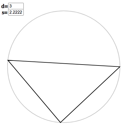
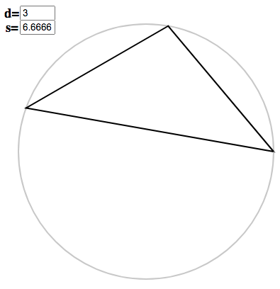
Tripling the argument gives $x = 6.\dot{6}$, which swings the points around to
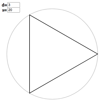
Tripling once more gives the last (genuinely regular) polygon:
Taking their tensor product, we have
To tote up the number of operations needed for the QFT, suppose it takes $O(n)$ gates to build an initial copygon, and that expansion is a single operation. Since we have $n$ factors, each starting with a copygon, and we expand $j$ times on factor $j$ (for $j \in [n]$), the total number of gates should be
\[nO(n) + \sum_{j=0}^{n-1} j = O(n^2) + \frac{1}{2}n(n-1) = O(n^2).\]If this operation takes $|s\rangle \mapsto |\chi^s_d\rangle$, then it acts on the full Hilbert space at no extra cost. By contrast, if we try to perform the QFT on the classical computer, we can still use (\ref{qft}) but cannot create a single circuit which computes everything at the same time. Instead, we need to laboriously compute individual Fourier coefficients $A_{-s}$, replacing $n$ parallelized computations of length $O(n)$ with $a^n$ classical coefficients involving $O(an)$ arithmetical operations. This changes the scaling to
\[O(a^{n+1}n),\]which is exponentially worse. Or, seeing this glass as half-full, the quantum computer is exponentially better! Although this is a nice heuristic for thinking about the $\text{QFT}_d$ and its gate complexity, it is not an algorithm, since we haven’t actually explained how to implement anything. For the conventional circuit description, see our final easter egg.
Algorithmic easter egg. Although it has the same scaling with $n$, building the initial copygon $n$ times is a massive duplication of effort. It is more economic to build each factor from scratch, and in this easter egg, we will explain in detail how. Since $d = a^n$ is a power of $a$, it is natural to expand $s$ in base $a$:
\[s = s_0 + s_1 a + \cdots + s_{n-1} a^{n-1}.\]We note that, modulo $a$, when we divide by a power $a^m$ for $m \leq n$, we get
\[\frac{s}{a^m} = \frac{s_0}{a^m} + \frac{s_1}{a^{m-1}} + \cdots + \frac{s_{n-1}}{a^{m-n+1}} \equiv \frac{1}{a^m}(s_0 + \cdots + s_{m}a^m) =: s_{(m)},\]since the higher powers give multiples of $a$. When written in base $a$, $s^{(m)}$ is just the expansion
\[s_{(m)} = s_m.s_{m-1} \ldots s_{0}.\]So we can rewrite the product (\ref{qft}) as
\[|\chi^s_{d}\rangle \simeq |\chi^{s_{(n-1)}}_{a}\rangle\otimes \cdots \otimes |\chi^{s_{(1)}}_{a}\rangle \otimes |\chi^{s_{(0)}}_{a}\rangle. \label{qft2} \tag{7}\]Recall that the QFT (\ref{qftd}) takes computational basis states to regular polygons. Here, we use the tensor basis, and make the natural extension of (\ref{kmn}):
\[|s(s_0, s_1, \ldots, s_{n-1})\rangle = |s_0 + s_1 a + \cdots + s_{n-1} a^{n-1}\rangle \simeq |s_0\rangle \otimes |s_0\rangle \otimes \cdots \otimes |s_{n-1}\rangle.\]Our goal is now to produce the factors in (\ref{qft2}) from these states. Let’s assume that the QFT on a module is a cheap operation, hardcoded into our quantum computer. From the first input state $|s_0\rangle$, we can use this to immediately get the first factor (from the right):
\[\text{QFT}_a |s_0\rangle = |\chi^{s_{0}}_{a}\rangle = |\chi^{s_{(0)}}_{a}\rangle.\]For the next factor, we once more apply the QFT:
\[\text{QFT}_a |s_1\rangle = |\chi^{s_{1}}_{a}\rangle,\]but this needs a correction from $s_1 \mapsto s_1.s_0$ (in base $a$). This is achieved by a controlled correction:
\[C^1|s_0\rangle |s_1\rangle = |s_0\rangle C^1(s_0)|s_1\rangle,\]where the matrix $C^1(s_0) = \mbox{diag}(\omega_a^{ks_0/a})$, where $k$ labels the diagonal entries. Let’s check this matrix does what we claim it does:
\[\begin{align*} C^1(s_0)|s_1\rangle & = \mbox{diag}(\omega_a^{ks_0/a}) \cdot \frac{1}{\sqrt{a}}\sum_k \omega^{ks_1}_a |k\rangle = \frac{1}{\sqrt{a}}\sum_k \omega^{k(s_1 + s_0/a)}_a |k\rangle = |\chi^{s_{(1)}}_{a}\rangle. \end{align*}\]So we’ve produced the second factor, and we didn’t “use up” $s_0$ while we were at it! It simply acted as a control bit and passed through. We can continue in this fashion, using the controlled operation
\[C^m |s_j\rangle = |s_j\rangle C^m(s_j), \quad C^m(s_j) := \mbox{diag}(\omega_a^{ks_j/a^{m}})\]to correct the $m$th digit in the base $a$ expansion. Schematically, we can put all this together and draw the circuit which performs $\text{QFT}_d$:
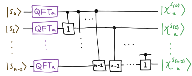
Control bits are indicated by black dots, and $C^m$ by a box labelled with $m$. Since this circuit gives the right answer for a basis element of the tensor product, by the magic of linearity, it works on the full Hilbert space. Technically, the final factors are in the wrong order, and to reverse these by, e.g., swapping adjacent wires, will take an extra $O(n^2)$ operations. The total number of gates required to implement the QFT with this circuit is then
\[n + \sum_{j=0}^{n-1} j + O(n^2) = \frac{1}{2}n(n+1) + O(n^2) = O(n^2),\]as we found above. Picturing the action of this circuit in terms of polygons is straightforward. Instead of expanding an initial copygon some number of times, we are building a polygon, then contracting it and adding a new term in the unit place of $x$:
\[s_0 \mapsto 0.s_0 \mapsto s_1.s_0 \mapsto 0.s_1s_0 \mapsto s_2.s_1s_0 \ldots\]These “controlled corrections” are a clever way to squish our old copygons.
4. Conclusion
Our initial motivation was to circumvent pesky evolutionary constraints on the visual cortex. To do this, we adapted a familiar grade-school method which (secretly) encodes infinite-dimensional vectors, namely graphs on the Cartesian plane. For a finite-dimensional complex vector, we drew a chain of points on the complex plane, and then joined the endpoints to obtain a marked directed polygon.
Our first task was to see how the standard basis elements looked. They were almost indistinguishable, which sucks. Rather than abandon our new toy, we decided to find a basis that looked better. Our polygonal representation suggested a basis of regular polygons, and either by direct computation, or group theory, we saw this choice worked. The QFT is simply the active change from the computational basis to this regular polygonal basis, and we found that the coefficients after the change of basis had a simple interpretation in terms of the hinged motion of a linkage.
Finally, we examined the effect of tensor factorization on the QFT, and discovered that it split a large regular polygon into smaller polygons spammed via “copygons”. Heuristically, the QFT builds the initial copygon and iteratively expands it on each factor. However, from a strict algorithmic point of view, it’s quicker to build the tensor factors in the other order, starting with a small polygon then iteratively squishing and adding digits. The corresponding quantum circuit takes exponentialy fewer operations than the best classical algorithm. So, by looking for pretty pictures of Hilbert space, we stumbled onto a massive algorithmic speedup! And they told you to stop doodling in math class.
References and acknowledgments
- Quantum Computation and Quantum Information (2000), Michael Nielsen and Isaac Chuang. Cambridge University Press.
- “Geometry and the Discrete Fourier Transform” (2010), Patrick Ion. American Mathematical Society monthly feature column.
Thanks to Olivia Di Matteo, Pedro Lopes and Rafael Haenel for feedback on this tutorial’s prior incarnations. Applets were made in p5.js and remain regrettably buggy. Finally, I’d like to acknowledge Acushla Burden for moral support, Yoshua Wakeham and Sarah Alexander for the gracious loan of a man cave, and Hudson Michael Laszlo Alexander-Wakeham for informative gurgles at key points.