This is the technical appendix to my post on napkin hacks. It contains solutions to exercises, and some material I deemed overly technical for the post. Very much under construction!
Contents
1. Solutions to exercises
1.1. Interplanetary pumpkins
1..2. Terminal raindrops
2. Technical results
2.1. Equilibrium for pollen grains
Prerequisites: familiarity with exponentials.
The equilibrium condition for pollen grains is more complicated than the simple equation I gave in the main text. If there are many balls of resin, they will settle at different heights, and the number of particles will change with height.
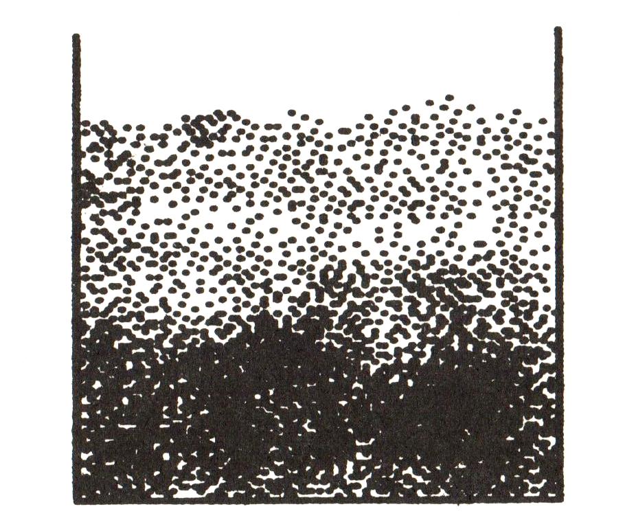
Nature likes low energy states. In a hot system, there is an element of randomness, but nature penalises high energy states by making them exponentially unlikely:
\[\text{probability}(E) \propto e^{-E/k_B\mathcal{T}}.\]They are not exactly zero, but when the energy $E$ is much greater than the thermal energy $k_B\mathcal{T}$, they may as well be! For a gas in a tall container, the energy is just the gravitational potential energy, $E = mgh$, and the number density of particles is proportional to the probability. The result is the barometric distribution:
\[n(h) = n_0 e^{-mgh/k_B\mathcal{T}},\]where $h = 0$ is the bottom of the container, and $n_0$ is a constant (with dimensions of density) that fixes the overall number of particles.
The barometric distribution tells us what the length $\ell = k_B\mathcal{T}/mg$ really means. Rather than being the mean free path (which changes with $h$), it is the approximate height over which the pollen or resin balls are concentrated; above $h = \ell$, they drop off exponentially. We could argue that $\ell$ is in some sense a typical distance between collisions, and leave it at that. But given that this is a technical appendix, we may as well work a bit harder! The correct approach comes not from equilibrium for an individual grain, but from dynamic equilibrium: the balancing act between resin balls falling under gravity, and randomly walking upwards. This will give us a deeper understanding of Brownian motion.
Consider a thin slice of the fluid at height $h$, with density $n$, thickness $\Delta h$ and area $A$. This slice will lose particles as they fall under the influence of gravity. In equilibrium, particles fall at the terminal velocity $v_\text{term}$, and hence the slice loses particles at a rate
\[R_\text{loss} = n A \Delta h v_\text{term}.\]But balls of resin also perform random walks. They will tend to wander from regions of high concentration to regions of low concentration, since (as discussed in the main text) a cloud of random walkers tends to spread out. Since the layer below will tend to have more resin balls (according to the barometric distribution), there will be a upward spread of walkers. We expect this will involve $\Delta n$, the difference in number density, and the rate of diffusion $D$. The rate of gain should then take the form (Exercise A.1)
\[R_\text{gain} = -D A \Delta n.\]Finally, in equilibrium, the rate of gain and loss are equal! Thus, we have that
\[n A \Delta h v_\text{term} = -D A \Delta n \quad \Longrightarrow \quad v_\text{term} = -\frac{D}{n}\frac{\Delta n}{\Delta h}.\]This looks complicated, but for the barometric distribution (Exercise A.2), it turns out that
\[\frac{1}{n}\frac{\Delta n}{\Delta h} = -\frac{mg}{k_B\mathcal{T}} \quad \Longrightarrow \quad v_\text{term} = \frac{Dmg}{k_B\mathcal{T}}.\]If we now plug in the terminal velocity from Stokes’ law, we can rearrange to find the Stokes-Einstein relation we derived (with considerable trickery) in the main text:
\[D = \frac{k_B\mathcal{T}}{6\pi \mu r}.\]There are various factors of $2$ we’ve neglected. But given the dimensional analysis-based sloppiness I’m advocating in general, we won’t lose sleep over them!
Exercise A.1 (grabbing granules). The rate at which a thin slice of fluid gains resin particles, $R_\text{gain}$, will involve:
- The difference in concentration $\Delta n$ between layers.
- The area $A$ of the layer.
- The diffusion constant $D$ for resin particles.
The rate $R_\text{gain}$ has dimensions of number per time. Find the dimensions of the terms in the list above, and conclude from dimensional analysis that
\[R_\text{gain} \sim -D A \Delta n.\]⁂
Exercise A.2 (exponential change). One way of defining an exponential is as the limit
\[e^x = \lim_{n\to\infty} \left(1 + \frac{x}{n}\right)^n.\]The binomial approximation says that for small $X$ (written $X \ll 1$), and any $\alpha$,
\[(1 + X)^\alpha \approx 1 + \alpha X.\]We can combine these two facts to learn something cool about the barometric distribution!
(a) Show using the binomial approximation that
\[e^x = \lim_{n\to\infty} \left[1 + x + x^2(\cdots)\right],\]where the $ \cdots$ denote terms multiplied by $x^2$.
(b) Using (a), argue that for $x \ll 1$,
\[e^x \approx 1 + x.\](c) The barometric distribution is
\[n(h) = n_0 e^{-mgh/k_B\mathcal{T}}.\]From the previous exercise, show that, if $\Delta h \ll k_B\mathcal{T}/mg$, then
\[\frac{\Delta n}{\Delta h} = \frac{n(h+\Delta h) - n(h)}{\Delta h} \approx -\left(\frac{mg}{k_B\mathcal{T}}\right) n(h).\]