March 11, 2020. This is a self-contained introduction to minimal networks (aka Steiner trees) in the plane. The first section discusses local geometric features, the second the structure of networks, and in the final section, what minimal networks can tell us about soap bubbles and vice versa.
Contents
1. Introduction
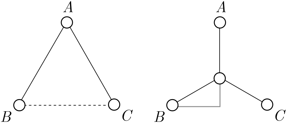
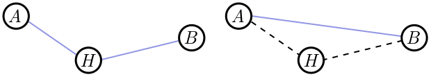
Suppose we want to join up three towns ($A$, $B$ and $C$) by rail. If I can use this railway to travel from one town to any other, we say that the rail network is connected. Two simple examples of connected networks are shown below.

Building railways is expensive, since we not only need to design and build the rail itself, but acquire the land beneath it. In contrast, stations are cheap: we just slap together some sidings, a platform, and a bench or two, and voila. To minimise cost, we should make the total length of the rail network as short as possible, adding extra stations if they help us do this. The resulting layout is called the minimal or Steiner network connecting $A$, $B$ and $C$.
We can consider the same problem for $n$ stations, and find the rail networks of smallest total length which connect them. Although finding the exact minimal network is difficult in general, we can derive some beautiful results about their geometry and layout. We step through the reasoning in bite-sized chunks, starting with the problem of connecting three cities.
Exercise 1 (choosing sides). Suppose $A$, $B$ and $C$ are separated by distances $AB = c$, $AC = b$ and $BC = a$. A triangular network consists of two sides of the triangle. Which ones should we choose?
⁂
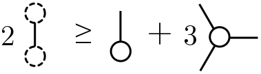
Exercise 2 (triangle or trident). In Figure 1, we have two networks connecting the same towns: a triangular network, and a trident-shaped network with a hub station $D$ in the middle. Which is shorter? See if you can do better than either.
Hint. Measure lengths on the screen with a ruler. Simple but it works!
2. Triangles
The three-town problem is already surprising. The simplest network consists of two sides of the triangle, but it is not minimal; to minimise length, a trident-shaped network, with a new hub station $D$ in the centre, is optimal. The best place to put the hub station is called the Fermat point, which you can find defined in various places online. But for the rest of the post, we will only worry about when we should build a hub, rather than where it goes exactly. This will save us some hard trigonometry! The one exception will be an important special case: the equilateral triangle.
2.1. Equilateral triangles
Suppose that the towns $A$, $B$ and $C$ sit on the corners of an equilateral triangle of side length $d$. The triangular network has total length $L_\Lambda = 2d$.
It seems plausible that the trident network does better, but instead of checking with a ruler, let’s do some basic trigonometry.
Exercise 3 (equilateral trident). Show that the length of the trident network, with a hub in the centre of the triangle, is
\[L_{\text{Y}} = \sqrt{3}d.\]Since $\sqrt{3} \approx 1.7 < 2$, the trident is indeed shorter than the triangle.
Hint. Use the grey triangle in Figure 2.
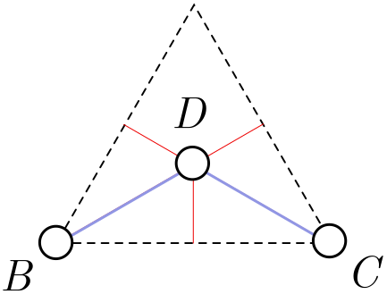
You might guess that the best place to put the hub station $D$ is right right in the centre, and in fact, we can prove this from symmetry. First of all, draw an axis of symmetry of the triangle, represented by the red line in Figure 3.
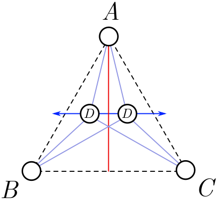
We are going to wiggle the hub side to side around this axis, along the dark blue line in Figure 3. From left-right symmetry, the length must either be a minimum or a maximum on the axis itself. Since the total nework length gets very large when we take the hub outside the triangle, it must be a minimum. So, for a minimal network, we must place $D$ on the red line.
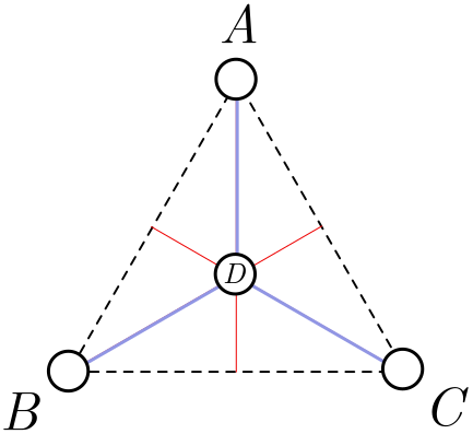
But there are axes of symmetry associated with $B$ and $C$ as well, and all three intersect at the centre of the triangle. Since $D$ should lie on each of these lines, it must lie at the centre! This completes our proof. The minimal network is depicted in Figure 4.
2.2. Deforming the triangle
We are now going to take our solution to the equilateral triangle and slowly deform it. In other words, we imagine slowly moving the corners of the triangle so it is no longer equilateral. What will happen to the optimal position of the hub $D$? Since everything is being smoothly modified, the position of the hub should change smoothly as well. In Figure 5, the smooth paths of the corners are depicted in purple, and the corresponding smooth change of hub in green.
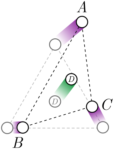
Since the hub position changes smoothly, it should stay inside the triangle for small deformations of the corners. But for triangles which are very far from equilateral, the hub might intersect one of the corners, and our trident network becomes a simpler triangular network, formed from two sides of the triangle.
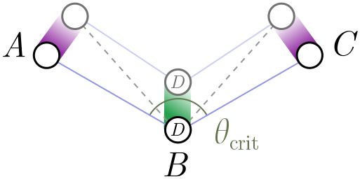
We picture this in Figure 6 above. In this diagram, $B$ remains fixed in position, but $A$ and $C$ slowly lower and open out the angle of the triangle, with the optimal hub $D$ moving down as they do so. At some critical angle $\theta_\text{crit}$, it will coincide with $B$. The question is: what is the angle?
It turns out this critical angle is $\theta_\text{crit} = 120^\circ$. Although we won’t provide a watertight proof, we can give a plausibility argument. Let’s return to the equilateral triangle. Instead of adding a hub in the middle, suppose that $D$ is in fact a fourth city fixed in place. Clearly, the solution in Figure 4 is still optimal, since if we could add more hubs to reduce the total length, we could add more hubs to improve the network for the equilateral triangle! If I now remove any of the corner cities $A$, $B$ or $C$, the optimal network simply removes the corresponding leg of the trident (Figure 7).
Exercise 4 (cutting corners). Suppose that in Figure 7, we can add a new hub $E$ which reduces the length of the network. Explain how adding $E$ could reduce the length of the network in Figure 7, and thereby improve our solution for the equilateral triangle.
Note. This is an example of a proof by contradiction. To show something is false, we assume it is true and use it to derive a contradiction with known facts. We then reason backwards to conclude that it cannot be true!
⁂
Exercise 5 (critical isosceles). The argument above really only establishes that $\theta_\text{crit} \leq 120^\circ$. It is possible, in principle, that the triangular network becomes shorter at some angle $\theta_\text{crit} < 120^\circ$. In this exercise, we will show for an isosceles triangle that this is not the case.
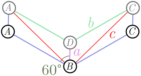
Figure 8 shows the triangular network (blue lines) $ABC$, forming an angle of $120^\circ$. We now raise the two nodes $A$ and $B$ at the end, so that the angle $ABC$ is less than $120^\circ$. You can prove that the green and purple lines are shorter than the red lines, so that an interior hub $D$ yields a shorter network.
(a) Show using the law of cosines (or otherwise) that
\[c^2 = a^2 + b^2 + ab.\](b) From part (a), show that
\[a + 2b < 2c.\](b) Conclude that for an isosceles triangle $ABC$, the critical angle is $\theta_\text{crit} = 120^\circ$.
2.3. Hubs and spokes
All this work with triangles pays off with a powerful conclusion for minimal networks connecting any number of cities:
In any minimal network, all hubs have three incoming legs separated by angles of $120^\circ$.
The argument is beautiful and simple.
Proof. Our first step is to show that it is impossible for a hub to have edges separated by less than $120^\circ$. Suppose we have cities $A_1, A_2, \ldots, A_n$ connected by a minimal rail network. Also suppose there is a hub station $H$ with incoming rail lines separated by less than $\theta_\text{crit} = 120^\circ$, as on the left in Figure 11. There may be other incoming lines (the horizontal lines in Figure 11), but these will play no role in our proof and can be ignored.
We can build two new stations on these outgoing legs, $h_1$ and $h_2$, which are (for simplicity) the same distance from $H$.
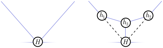
It’s easy to see that every angle in this triangle is less than $120^\circ$, since the angles at $h_1$ and $h_2$ are at most $90^\circ$, and we’ve assume the angle at $H$ is less than $120^\circ$. Thus, from our work in the previous section, we know that the minimal network connecting $h_1$, $h_2$ and $H$ is not the triangle we have drawn, but a trident with another hub $h_3$ in the middle! This strictly decreases the length of the network (shown right in Figure 9), and hence, our original network must not have been minimal. There’s our contradiction!
So, we know that any hub must have spokes separated by at least $120^\circ$. How do we know that there are three, separated by exactly $120^\circ$? This is very simple. Suppose two lines enter $H$, separated by more than $120^\circ$. Then there can only be two incoming edges, joining $H$ to some cities $A$ and $B$, since any additional lines would have to be closer than $120^\circ$ to one of these lines, given the result we just proved. So, we have the situation depicted on the left of Figure 10:
Hopefully you can see what goes wrong. If there is a “kink” in the line, with separating angle $\theta \neq 180^\circ$, then we can obtain a shorter network be deleting $H$ and directly connecting $A$ and $B$. Once again, we have a contradiction!
Now, strictly speaking, we can have hubs with only two incoming edges, separated by $180^\circ$. But such a hub is always unnecessary, since all it does is sit on a straight line. In real life, hubs do cost some money (even if it is dramatically less than spokes) so we will never build unnecessary ones! If we always delete these useless hubs, we have the general result advertised above, namely that any hub in a minimal network has three equally spaced spokes.
Exercise 6 (outer rim). Our proof applies to hubs only, but the same style of argument allows you to deduce properties of the cities or fixed nodes $A_1, A_2, \ldots, A_n$. Prove the following properties:
(a) No incoming edges can be separated by less than $120^\circ$.
(b) The number of incoming edges is between $1$ and $3$.
(c) A city has three edges only if it lies at the centre of an equilateral triangle of nodes.
The upshot is that the fixed nodes can have from one to three edges, with three only in special circumstances.
⁂
Exercise 7 (easy polygons). Consider cities on the corners of a regular $n$-gon. Show that for $n \geq 6$, the minimal network is just the perimeter with one edge removed.
3. Graphs
In this section, we will learn more about the connectivity and layout of minimal networks. The geometry we learned in the last section will be essential!
3.1. Trees
In a minimal rail network, how many ways can I get from $A$ to $B$? If the network is connected, then the answer is at least one. That’s the definition of connected! But if the network is minimal, the answer is exactly one. If there is more than one way to get from $A$ to $B$, the network has unnecessary edges and can be pruned to get something shorter. We might worry that pruning redundant paths between $A$ and $B$ could disconnect other cities, but this is never the case. Figure 11 shows why.
Suppose $A$ and $B$ are connected by two paths, labelled $1$ and $2$. The green blob to the left is all the nodes whose paths to $B$ go through $A$ first, and similarly, nodes on the right connect to $A$ through $B$. If two nodes are in the same blob, such as $C$ and $E$, then pruning path $2$ has no effect on whether they are connected. If two nodes are in different blobs, like $C$ and $D$, they can still reach each other using path $1$. So, pruning redundant paths between $A$ and $B$ does not affect whether other nodes connect.
Exercise 8 (path pruning). Generalise the argument above to account for nodes that lie between $A$ and $B$. More precisely, these are nodes which can connect to either $A$ or $B$ without passing through the other, and schematically lie on paths $1$ or $2$.
Once we have completely pruned the network, there is only a single path connecting any two nodes $A$ and $B$. Such a network is called a tree because of the way it branches. For this reason, minimal networks are more often called Steiner trees. An example is shown in Figure 12.
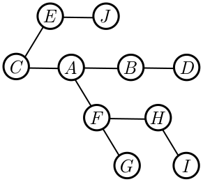
Our reasoning shows that minimal networks are trees. The number of nodes in the network is $N = n + h$, where $n$ is the number of fixed nodes and $h$ counts the hubs added to make the network as short as possible. In Figure 12, for instance, we have $N = 10$. The number of edges $E = 9$ is one less than the number of nodes. This is not a coincidence, and for any tree, it turns out that $E = N - 1$. To prove this, we first need to know that (unlike real life), in graph theory, every tree has leaves.
Exercise 9 (trees and leaves). A leaf is a node with a single edge, e.g. the nodes $J$, $D$, $G$, and $I$ in Figure 12. Part (a) will show what we need, namely that every tree has a leaf, and parts (b) and (c) probe this question a little more deeply. To begin, we will choose a node at random (red in Figure 13) and count the number of steps to each other node. Since there is a unique path between two nodes in a tree, this is well-defined.
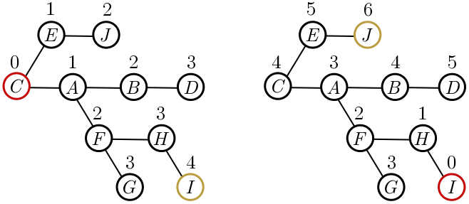
(a) Consider the node or nodes furthest from our selected node (orange nodes in Figure 15). Argue that these must be leaves. Hint. If they are not, what are the distances of the neighbours?
(b) Take the furthest node and now find the node or nodes furthest from it. Argue that these are also leaves, and conclude that every tree has at least two leaves.
(c) Show, using an example, that a tree need not have more than two leaves.
The procedure for finding leaves is illustrated in Figure 15. We start with an arbitrarily chosen node $C$, and calculate distances to all other nodes. The most distance node is $I$, which is indeed a leaf. Measuring from $I$, the most distant node is $J$, which is also a leaf.
We now know that every tree has a leaf. If we remove it, and the single edge connecting it to the rest of the graph, we decrease the number of nodes and edges by $1$, $N \to N- 1$ and $E \to E - 1$. We keep doing this until we are down to a single node. This has no edges at all, and since we decrease by $N-1$ nodes to obtain a single node, decreasing $E$ by the same amount gives $0$. Hence, for trees in general,
\[E = N - 1.\]3.2. Bounding hubs
If we combine our geometric results from earlier with our result about trees, we can constrain the layout of minimal networks further. Recall that each of the $h$ hubs (once we delete the useless ones) has exactly three edges. Each of the $n$ fixed nodes has at least one edge to ensure it is connected to the rest of the network. Thus, the total number of edges $E$ obeys the inequality
\[E \geq \frac{1}{2}\left(n + 3h\right).\]In diagrams,
The factor of $2$ occurs because we are counting edges twice in the leftmost and rightmost expression: each end of an edge is associated with a vertex, and we are counting the contribution at each vertex once. From the previous section, we know that $E = N - 1$. This gives
\[\frac{1}{2}\left(n + 3h\right) \leq N - 1 = n +h - 1.\]After some algebra, we find that
\[h \leq n - 2.\]The maximum number of hubs $h = n - 2$ is achieved when each fixed point has precisely one edge. In this case, the leaves of the graph are exactly the fixed nodes.
3.3. Tinkertoys
Combining the geometry and graph results gives us a simple tool for building minimal networks. For $n$ fixed nodes, pick $h = n-2$ hubs, with spokes emerging at angles of $120^\circ$, and connect them together to form a tree. We call this configuration of hubs and spokes a tinkertoy. It is almost rigid, but we can extend the spokes and legs. For $h = n-2$, the minimal network is always a tinkertoy, but see Exercise 10 for an example of a minimal network which is not.
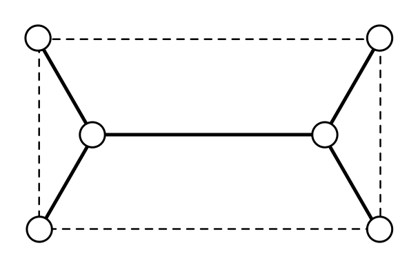
Let’s illustrate the tinkertoy approach for fixed nodes on a rectangle. There is only one tinkertoy, connecting the closest external nodes in pairs, as shown in Figure 14.
The situation for a general quadrilateral is a bit trickier, but can be quickly solved by a computer fiddling with the tinkertoy.
Exercise 10 (minimal network on a rectangle). A rectangle has width $w$ and height $h$, with $w \leq h$. Show that the minimal network has length
\[L = w + \sqrt{3}h.\]⁂
Exercise 11 (harder polygons). When $h= n-2$, you can use a single tinkertoy, but if $h < n - 2$, you will need multiple tinkertoys. Here we give examples of both.
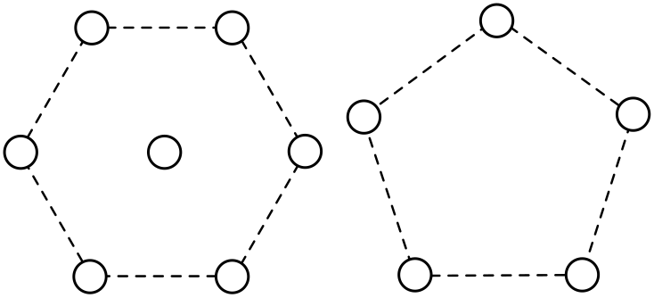
(a) Find the minimal network connecting a regular hexagon with a node in the centre. (To be clear, this central node is fixed.) You will need multiple tinkertoys!
(b) Draw the tinkertoy for a regular pentagon, and schematically indicate what the minimal network looks like.
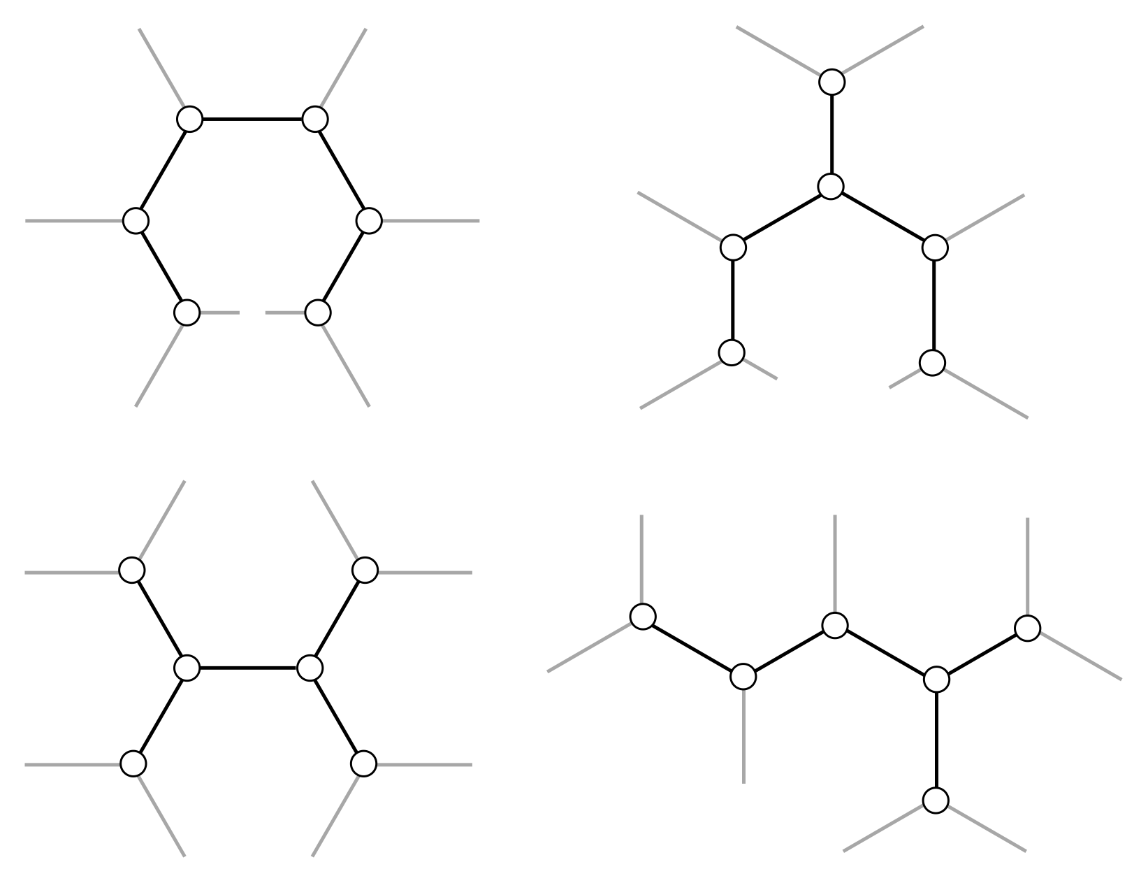
For a small number of fixed nodes, tinkertoys are useful. But how useful are they for many nodes? Let’s assume that fiddling with tinkertoys is a quick operation, and we can tell after some fixed time (independent of $n$) whether a particular tinkertoy can connect the fixed nodes. Unlike the cases we’ve look at so far, for large $n$, there are many different tinkertoys to try out. For instance, we show the four different tinkertoys for $h = 6$ (or $n = 8$) in Figure 16.
In Exercise 12, you’ll prove that there are exponentially many tinkertoys with $h$ hubs as $h$ gets large. A brute force approach, which simply checks each tinkertoy, will take an exponential amount of time, and since exponential get large very quickly, this approach is not computationally feasible for large $h$. Unfortunately, there are no algorithmic shortcuts! You can eliminate some tinkertoys from consideration, but as $n$ gets large, there will always be fixed nodes which require you to try an exponential number. This makes the mathematical solution of the minimal network effectively impossible to compute.
Exercise 12 (counting tinkertoys). Counting the precise number of tinkertoys $T_h$ for any number of hubs $h$ is difficult. But we can cheat in two different ways: show that $T_h$ is greater than some exponentially growing sequence, $S_h$; or use “physicist’s induction”, where we calculate for small $h$ and guess the rest of the sequence.
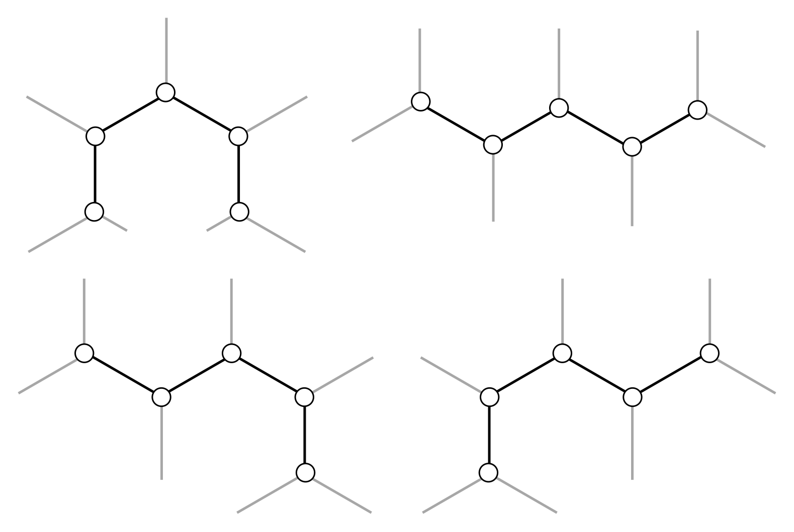
(a) Consider the set of “snake” tinkertoys, where hubs are connected in a single line. Show that, for $h \geq 3$ hubs, there are $S_h = 2^{n-3}$ snake tinkertoys. Since $T_h \geq S_h$, this demonstrates that the total number of tinkertoys grows exponentially.
(b) Calculate the number of tinkertoys from $h = 0$ to $h = 6$. You should be able to find the general sequence $T_h$ by looking for these numbers in the Online Encyclopedia of Integer Sequences. At large $h$, this sequence is indeed exponential, with
\[T_h \approx \frac{2^{2n-4}}{\sqrt{\pi}h^{5/2}}.\]4. Soap bubbles
Humans are not the only players in the minimisation game. Nature also likes to minimise, and has far more power at her disposal than us mere mortals! While we struggle with tinkertoys, Nature can solve our problems, to good approximation, as effortlessly as a ball falls to the ground. We’ll start by thinking about soap bubble networks in general, and finish by describing soap bubble computers to help us find minimal networks.
4.1. Bubble networks
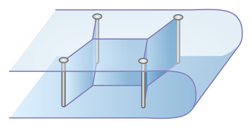
Bubbles are formed when a film of liquid separates two volumes of air. Surface tension tries to pull the bubble surface taut in all directions, which results in the minimisation of area. A soap bubble is spherical, for instance, since this is the smallest surface containing a fixed volume of air. If we attach two plexiglass plates together and dip them in soapy water, a two-dimensional network of bubbles with vertical walls will form. A single bubble will now be a cylinder, rather than a sphere, as in Figure 18.
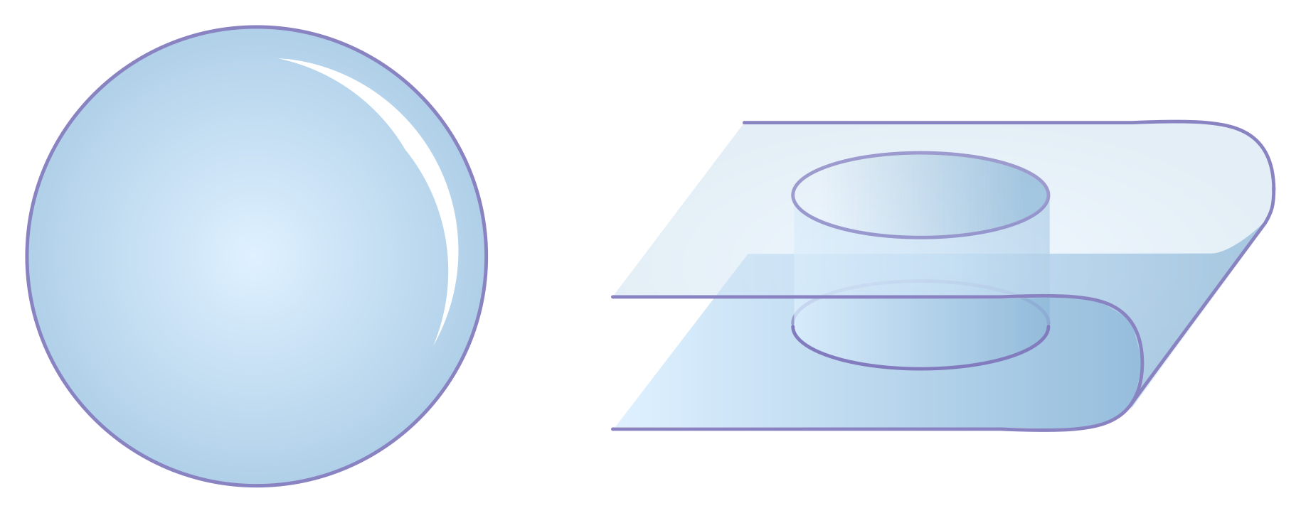
Typically, bubbles will form closed loops and hence are not minimal networks in our sense, since we explicitly ruled out loops earlier. But bubbles are locally minimal, in the sense that surface tension will tug on bubble walls, and reconfigure small bubbles, until doing so cannot reduce the area. And the result we found earlier, that hubs have three equally separated spokes, is a local condition, since it applies in the small region around a node! This means that in bubble networks, the same property is true: bubble walls always meet in sets of three, separated by $120^\circ$. This even applies to curved bubble walls (which arise from pressure differences), since when you zoom in on a junction these curved walls look straight.
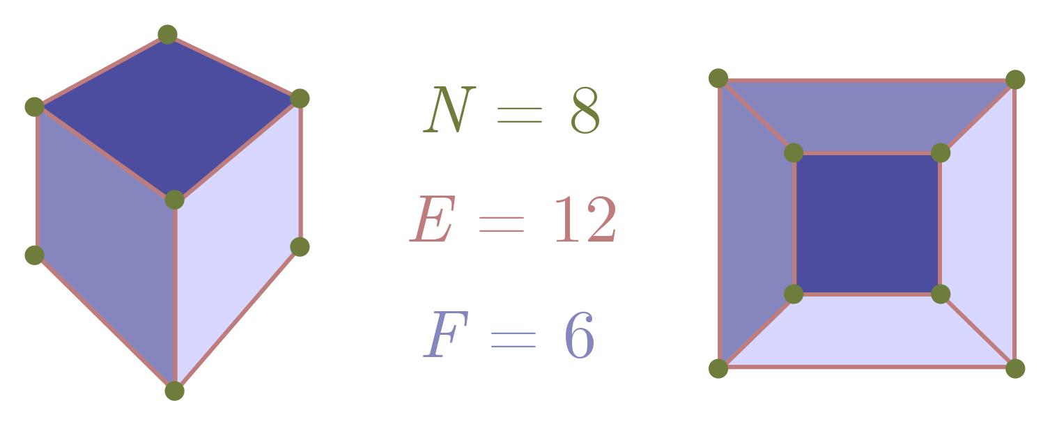
We can use this to explain why two-dimensional foams form hexagons! We don’t need any physics, just the result about hubs, some network theory, and a few reasonable assumptions about what happens as a foam network gets bigger. The main fact about network theory is Euler’s formula, governing the relationship between nodes $N$, edges $E$, and faces $F$ in a graph:
\[N - E + F = 2.\]This relation is illustrated for a cube in Figure 19. Note that, for a graph, we count the whole region outside the network as a face! Exercise 14 guides you through a proof of this formula.
Now, for a two-dimensional foam, there are no “external” nodes. Each node is a hub, with three edges, so
\[2E = 3N,\]where we include the factor of $2$ as usual because of double counting. Putting this into Euler’s formula, we can eliminate $N$ and find a relation between the number of faces and number of edges:
\[\frac{2}{3} E - E + F = 2 \quad \Longrightarrow \quad 3F - E = 6.\]As advertised, we can treat the external face a little differently. Let’s call the internal faces $F’$, so that $F = F’ + 1$. Rewriting in terms of $F’$, we get $3F’ - E = 3$.
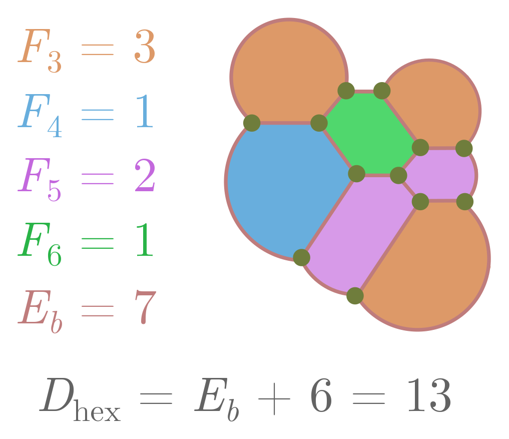
What has all this got to do with hexagons? Let’s introduce a number $F_s$ which counts the number of internal faces with $s$ sides, and $E_b$ stand for the number of edges of the outer face. Since we need at least one side to form a face, the total number of internal faces is
\[F' = F_1 + F_2 + F_3 + \cdots \,.\]But since each edge is associated with two faces, we can also express edges in terms of these numbers:
\[2E = E_b + 1 \cdot F_1 + 2 \cdot F_2 + \cdots + s\cdot F_s + \cdots \,.\]Since the $F_s$ only count the internal faces, and each external edge will be adjacent to one internal face. If we plug these expressions into $3F’ - E = 3$ and multiply everything by two, we finally get
\[6 + E_b = 6F' - 2E + E_b = (6-1) \cdot F_1 + (6-2) \cdot F_2 + \cdots + (6-s)\cdot F_s + \cdots \,.\]On the LHS, we have a term involving the number of external edges $E_b$. On the RHS, we have the difference from hexagonality, which we’ll call $D_\text{hex}$. For a face with $s$ sides, $6-s$ tells you how different it is from a hexagon! So, more simply, we have
\[D_\text{hex} = 6 + E_b.\]There are a few cute things we can learn from this expression. First of all, the LHS is positive, so $D_\text{hex} \geq 0$. The number of “small” faces $F_1, \ldots, F_5$ places a strong constraint on the number of “large” faces $F_7, F_8, \ldots$, and so on:
\[5 \cdot F_1 + 4 \cdot F_2 + \cdots + 1\cdot F_5 \geq + 1 \cdot F_7 + 2\cdot F_8 + \cdots \,.\]So if I count the number of small faces, I can immediately figure out the maximum number of large faces!
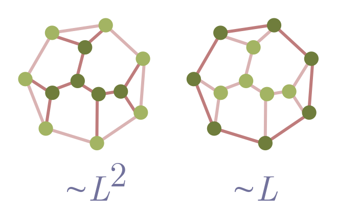
But our main goal was to show that foams are approximately hexagonal, so let’s proceed. Suppose the foam has size $\sim L$, where $L$ is some length scale like the radius, and $\sim$ means “scales as”. Then, assuming bubbles have a typical size independent of $L$, the number of external edges $E_b \sim L$. For instance, if bubbles have average edge length $\ell$, independent of $L$, and we have a circular foam of radius $L$, then $E_b = (\pi/\ell)L$. It follows that, for large $L$,
\[D_\text{hex} = 6 + E_b \sim L.\]The “density” of difference from hexagonality $d_\text{hex}$ is just the total difference divided by the area of the foam. This should scale as $L^2$, so that
\[d_\text{hex} \sim \frac{D_\text{hex}}{L^2} \sim \frac{1}{L}.\]As the foam becomes larger, differences from hexagonality become increasingly rare! A typical bubble in a two-dimensional foam has six sides. You can repeat the argument, but for a set of contiguous bubbles in a larger foam, in Exercise 13.
Exercise 13 (bubble blobs). A “bubble blob” is a set of contiguous bubbles in a (two-dimensional) foam. Let $E_o$ denote the number of edges extending outward from the boundary, and $E_i$ the number extending inward.
(a) Explain why the difference from hexagonality is now
\[D_\text{hex} = 6 + E_i - E_o.\](b) Repeat the scaling argument above, and conclude that in a large blob, departures from hexagonality become harder and harder to find.
⁂
Exercise 14 (Euler’s formula). Our goal here will be to prove Euler’s famous formula:
\[N - E + F = \chi = 2,\]where $N$ is the number of nodes, $E$ the number of edges, and $F$ the number of faces, in a network where edges do not cross. We have also defined $\chi = N - E + F$, called the Euler characteristic, for notational convenience. Although we are discussing this in the context of graphs, it holds in general for three-dimensional polyhedra like cubes and dodecahedra. In fact, the two are equivalent, since we can always flatten a polyhedron to get its net, which is a network.
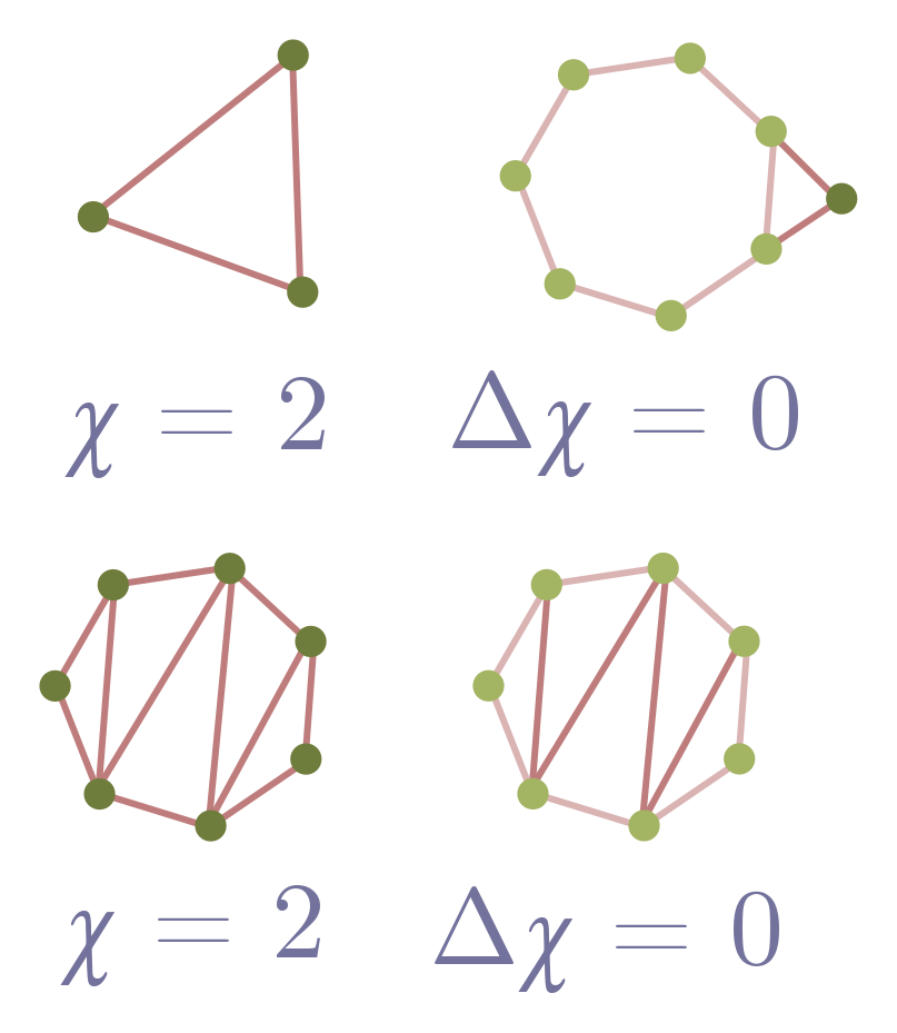
First, we will establish Euler’s formula for networks made out of triangles.
(a) Show that a lone triangle in the plane obeys Euler’s formula. Remember, we count the area outside the triangle as a face!
(b) Suppose I have a network which obeys Euler’s formula. Add a triangle (two edges and a node) to an external edge, and explain why the Euler characteristic doesn’t change, $\Delta \chi = 0$. Conclude that the new network obeys Euler’s formula.
(c) Explain why any network composed entirely of triangles obeys Euler’s formula.
Now, we can generalise to any network without crossings.
(d) Consider a face, i.e. loop, in such a network. Describe a procedure to add edges so that the face is split into triangles.
(e) Show that, after your procedure in part (d), $\Delta \chi = 0$.
(f) Combine your results to conclude that any network without crossings obeys $\chi = 2$.
4.2. Soap bubble computers
Soap bubbles find local minima quickly because of the laws of physics. Can we somehow “hack” soap bubbles, and turn them into analogue computers which find Steiner trees? Sort of. Computer scientist Scott Aaronson has persuasively argued that hard problems (such as finding Steiner trees) cannot be solved quickly, in the general case, by any physical mechanism. So as a matter of physical principle, we should not expect soap bubbles to quickly find arbitrary minimal networks.
But this doesn’t prevent soap bubbles from giving quick and correct solutions to some problems, nor does it forbid them from approximating the answer. Indeed, there are quick approximation algorithms for regular computers, so we shouldn’t be surprised if soap bubbles can do the same. So, can we quickly (and perhaps approximately) find minimal networks by dipping them in soapy water? The answer is yes!
The key is to give the bubble walls something to hold onto (Figure 23). In a foam, they can only hold onto themselves, and we get the non-crossing bubble networks described above. But if we drill some screws through the plexiglass, these will act like fixed nodes, and walls can form between these screws and hubs arising from the junction of three bubble walls. This analogue computer isn’t perfect, since the soap bubbles can converge on a locally minimal tinkertoy which connects the screws, but is not globally minimal. But it really is a lucky dip, and you can sometimes strike the true minimum, particularly for smaller problems where only one tinkertoy works. See this video for a demonstration, and the classic What is Mathematics? for discussions of how soap bubble computers can be applied to other mathematically difficult problems.
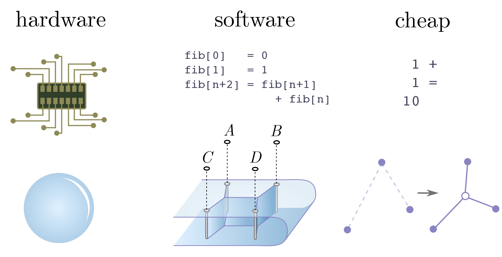
Soap bubbles do not magically solve problems thought to be impossible. But they do demonstrate strikingly that physical objects are computers, and the laws of physics do computational work. To expand on this statement, let’s consider the traditional division of computers into hardware and software. Hardware is the physical substrate the computer is built on. It tells us which operations are basic, and therefore computationally cheap. Software is a layer of instruction and abstraction above the hardware, telling the computer how to represent data and manipulate it to do useful things.
In the soap bubble computer, the hardware is clearly the bubbles themselves, and local area minimisation a cheap operation by virtue of the laws of physics. The software is nothing more complicated than drilling screws, dipping, and waiting for bubbles to form. In terms of computers built out of physically interesting hardware, this is just the tip of the iceberg! One of the big technological revolutions now in the progress is the advent of quantum computing, leveraging the weirdness of quantum mechanics. Perhaps more surprisingly, there is a sense in which black holes, DNA, and animal brains are all analogue computers, like the soap bubbles, with certain cheap operations. There are more computers in heaven and earth than are dreamt of in our philosophy!
Exercise 15 (trains and soap bubbles). The first mathematician to consider minimal networks on four points was the great Carl Friedrich Gauss (1777 – 1855). In an 1836 letter to his friend, the astronomer Schuhmacher, Gauss asked:
How can a railway network of minimal length which connects the four German cities Bremen, Harburg, Hannover, and Braunschweig be created?
The cities are drawn in Figure 25:
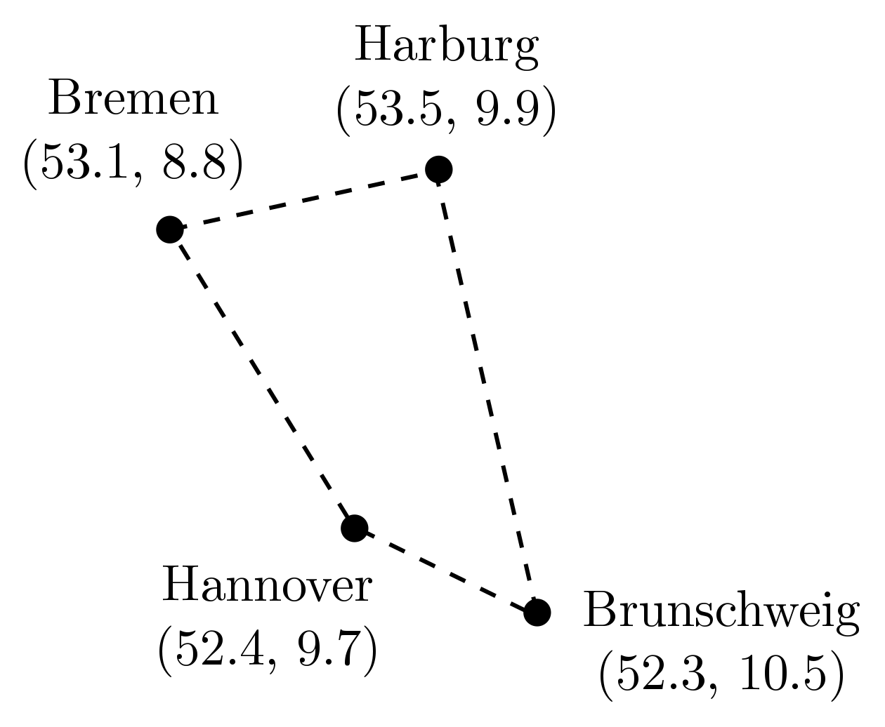
Your task is simple: build a soap bubble computer, and use it solve the original rail network problem! Figure 25 also gives the GPS coordinates, which you may find useful in placing your screws.
Acknowledgments
I’d like to thank Rafael Haenel, Pedro Lopes and Haris Amiri for feedback, and Rafael particularly for his encouragement. Some of this material was tested at the UBC Physics Circle, as part of a workshop run by Geering Up and Diversifying Talent in Quantum Computing, so I would also like the students for their participation and feedback!
References
- “NP-complete problems and physical reality” (2005), Scott Aaronson.
- What is Mathematics? (1941), Richard Courant and Herbert Robbins.
- “The Steiner minimal tree” (2015), Peter Lynch.
- “Structural Hierarchy” in Aesthetics in Science (1981), Cyril Stanley Smith.