July 28, 2019. Imaginary time is a trick for turning heat into geometry. More precisely, hot systems repeat themselves in imaginary time. This perspective leads to a quick proof of the Unruh effect (empty space looks hot when you accelerate) and with a little more work, to Hawking radiation (black holes are hot since observers near the horizon accelerate).
Introduction
Prerequisites: quantum mechanics, statistical mechanics, special relativity.
Thermodynamic systems, like light bulb filaments, puddles, or stars, consist of many components interacting at random. Rather than predict what will happen exactly, it makes more sense to consider what will happen on average. “Average” implictly requires a probability distribution, but all sensible choices yield the same result when there are many particles.
It’s easiest to work in the canonical ensemble, where the temperature $T$ is fixed. High energy states are exponentially unlikely, with
\[p_\beta(E) \propto e^{-\beta E}\]for $\beta = 1/k_B T$. This exponential is called a Boltzmann factor. We can immediately write down the full probability distribution over energy eigenstates, using the fact it is unit normalised:
\[p_\beta(E) = \frac{1}{Z[\beta]}e^{-\beta E}, \quad Z[\beta] = \sum_{E} n(E) e^{-\beta E}.\]Here, $n(E)$ is the density of states, telling us how many states have energy $E$. The normalisation factor $Z[\beta]$ is called the partition function, and it neatly encodes all the statistical properties of the system. For instance, the average energy of the system is a derivative of the partition function:
\[\langle E \rangle = \sum_E n(E) p_\beta(E) E = \frac{\sum_E n(E) e^{-\beta E} E}{\sum_E \rho(E) e^{-\beta}} = \frac{-\partial_\beta Z[\beta]}{Z[\beta]} = -\partial_\beta \ln Z[\beta].\]Another example is the Helmholtz free energy $F = -k_\text{B} T \ln Z[\beta]$, which quantifies the tradeoff between energy and entropy and is minimised in equilibrium.
Quantum statistical mechanics
The canonical ensemble also describes a quantum mechanical system at finite temperature, This is now a probability distribution over quantum states, with high energy states suppressed by Boltzmann factors:
\[\hat{\rho}_\beta = \frac{1}{Z[\beta]}\sum_E e^{-\beta E}|E\rangle\langle E|.\]Here, we are using Dirac’s bra-ket notation, and $|E\rangle\langle E|$ projects onto the energy eigenstate $|E\rangle$. Instead of having unit norm, the density $\hat{\rho}_\beta$ is defined to have unit trace:
\[1 = \mbox{Tr}[\hat{\rho}_\beta] = \frac{1}{Z[\beta]}\sum_E e^{-\beta E}\mbox{Tr}|E\rangle\langle E|= \frac{1}{Z[\beta]}\sum_E e^{-\beta E}.\]The normalisation $Z[\beta] = \sum_E E^{-\beta E}$ is a classical sum over Boltzmann factors, just like the classical case.
There is a nicer way to write the density $\hat{\rho}_\beta$. An energy eigenstate is an eigenvector of the system’s Hamiltonian (energy operator) $\hat{H}$, with $\hat{H}|E\rangle = E|E\rangle$. But by a standard linear algebra trick, we can write any diagonalisable operator as a sum of projectors onto its eigenvectors, weighted by eigenvalues:
\[\hat{H} = \sum_E E |E\rangle \langle E|.\]It follows that
\[\hat{\rho}_\beta = \frac{1}{Z[\beta]}e^{-\beta \hat{H}}, \quad \mbox{Tr}[e^{-\beta \hat{H}}] = Z[\beta].\]So the density and partition function have simple expressions in terms of the Hamiltonian.
Amplitudes and Wick rotation
The bridge between thermodynamics and imaginary time is the Hamiltonian. First, recall the Schrödinger equation for the evolution of a state $|\psi\rangle$,
\[i\hbar \partial_t |\psi(t)\rangle\]This is simple to solve when the Hamiltonian itself is time-independent:
\[\hat{H}|\psi(t)\rangle \quad \Longrightarrow \quad |\psi(t)\rangle = e^{-i\hat{H}t}|\psi(0)\rangle.\]We call $e^{-i\hat{H}t} = U(t)$ the propagator. The amplitude for a system to go from state $|\phi\rangle$ to $|\varphi\rangle$ in time $t$ is just
\[\langle\phi|U(t)|\varphi\rangle,\]since $U(t)$ updates the state, and the overlap with the bra $\langle\phi|$ tells us “how much” of $|\phi\rangle$ is in the evolved state $|\varphi(t)\rangle$. The return amplitude for a state $|\phi\rangle$ is just the amplitude for returning to the state a time $t$ later:
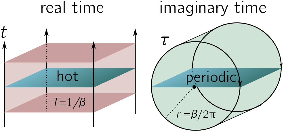
\[\langle\phi|U(t)|\phi\rangle.\]Now for a turn the screw. Define imaginary time by $\tau = i\tau$. This is called Wick rotation, since we can imagine multiplying by $i$ as rotating by $\pi/2$ in a complex plane for time. The propagator in imaginary time exponentially suppresses things:
\[U(-i\tau) = U_\text{im}(\tau) = e^{-\hat{H}\tau}.\]This smells like a Boltzmann weight! In fact, for an energy eigenstate $|E\rangle$, the imaginary return amplitude is precisely a Boltzmann weight:
\[\langle E| U_\text{im}(\tau) | E\rangle = e^{-E \tau}.\]We can reinterpret the density matrix in terms of these imaginary return amplitudes. Instead of viewing it as a probability distribution over energy eigenstates, we can interpret $\hat{\rho}_\beta$ as projecting onto a system which always returns to itself after imaginary time $\beta$, i.e. is periodic in imaginary time.
Concretely, whenever we evaluate some observable $\hat{A}$ in thermal state, the expectation is
\[\langle\hat{A}\rangle_\beta = \frac{\sum_E \langle E|e^{-\beta\hat{H}}\hat{A}|E\rangle}{Z[\beta]}.\]The numerator is the sum of expectations over all ways the system can return to its initial state after imaginary time $\beta$. The normalisation is the amplitude for this imaginary periodicity property. The whole expectation, then, takes the form of a conditional expectation in a state with imaginary periodicity, using an analogy with conditional probabilities:
\[\mathbb{P}(A|B) = \frac{\mathbb{P}(A\cap B)}{\mathbb{P}(B)}.\]Exercise 1. Statistical and quantum mechanics.
-
When there are many particles in the system, the sum in the canonical ensemble tends to be dominated by a single energy $E^*$, where the probability is concentrated. Argue that the free energy
\[F = -k_\text{B}T \ln Z[\beta] \approx E^* - T S(E^*),\]where $S(E) = k_\text{B}\ln n(E)$ is the entropy. This explains the more common definition of Helmholtz free energy as $F = E - TS$.
-
Prove the claim about the canonical density matrix above, i.e.
\[\hat{\rho}_\beta = \frac{1}{Z[\beta]}e^{-\beta \hat{H}}, \quad \mbox{Tr}[e^{-\beta \hat{H}}] = Z[\beta].\]You can use the result (true for spectral decompositions in general) that
\[e^{\lambda \hat{H}} = \sum_E e^{\lambda E}|E\rangle\langle E|.\] -
Derive the simple expression for the thermal expectation, $\langle\hat{A}\rangle_\beta = \mbox{Tr}[\hat{\rho}_\beta\hat{A}]$.
Rindler coordinates and the Unruh effect
Let’s now turn from quantum mechanics to special relativity. To keep life simple, we stick to two dimensions with Minkowski coordinates $(t, x)$. Recall that the signed distance $s^2$ from the origin to a point in spacetime $P(t, x)$ is given by
\[s^2 = -t^2 + x^2.\]For small displacements, this defines the Minkowski metric
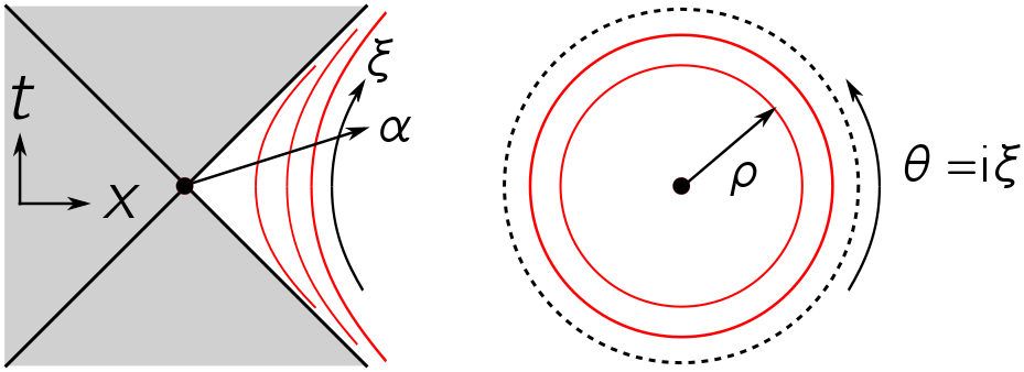
\[ds^2 = -dt^2 + dx^2.\]The curves at fixed distance $s^2 > 0$ from the origin are hyperbolas covering the east-west quadrants. We can use these hyperbolas to define a new coordinate system on, say, the east quadrant:
\[x = \alpha^{-1} \cosh\xi, \quad t = \alpha^{-1} \sinh\xi.\]Note that $s^2 = \alpha^{-2}$ on a hyperbola, and $t = x \tanh\xi$ for fixed $\xi \in \mathbb{R}$. Thus, we can draw our coordinates as follows:
Exercise 2. Rindler coordinates.
- Verify the geometric description of $\alpha, \xi$ above.
- For an observer on a fixed hyperbola labelled by $\alpha$, verify that their proper time is $\alpha \xi$ and their proper acceleration has magnitude $\alpha$. This gives a second way of interpreting Rindler coordinates.
-
Show that the Minkowski metric in Rindler coordinates is
\[ds^2 = -\frac{1}{\alpha^2}d\xi^2 + \frac{1}{\alpha^4} d\alpha^2.\] -
Defining $\rho = 1/\alpha$, show that the metric takes the simple form
\[ds^2 = -\rho^2\, d\xi^2 + d\rho^2.\]
To understand the thermal properties of Rinder coordinates, we go to imaginary time, $\xi = -i \theta$. This leads to the metric
\[ds^2 = \rho^2\, d\theta^2 + d\rho^2.\]This is precisely the metric on a disk, with radius $\rho$ and polar angle $\theta$. If this language of metrics is confusing, we can see it explicitly from the change of coordinates:
\[x = \rho \cosh(-i\theta) = \rho\cos\theta, \quad \tau = it = i\rho \sinh(-i\theta) = \rho \sin\theta.\]Of course, the period in imaginary time depends on whether we choose $\tau$, $\theta$, or the imaginary proper time $\alpha\theta$. It turns out that temperature is in the eye of the beholder, and we must choose the imaginary proper time to determine the energies they will measure. Since the proper time is $\alpha\xi$, the period in proper imaginary time is $2\pi \rho$. Recalling our mantra, we are led to predict that the “system” — empty space — appears thermal, with temperature
\[T_\text{U} = \frac{\alpha}{2\pi}.\]The fact that empty space looks thermal to an accelerating observer is called the Unruh effect, and $T_\text{U}$ the Unruh temperature. If we restore the factor of $\hbar$ omitted from Schrödinger’s equation, the factor of $k_\text{B}$ omitted from the inverse temperature $\beta$, and the factor of $c$ omitted from the Minkowski metric, we get the expression
\[T_\text{U} = \frac{\hbar \alpha}{2\pi k_\text{B} c}.\]In our earlier quantum mechanics discussion, a thermal density arose from having a geometry with imaginary periodicity. For the same reason, when we go to define quantum fields on the imaginary Rindler spacetime, they will be in a thermal state. To show this is true requires a discussion of what is called the path integral approach to quantum field theory and quantum mechanics, which is beyond our scope here. But the arguments work in a very similar (if slightly more technical) fashion, and the conclusions are the same: the accelerating observer will see a thermal bath of particles, such as photons and any other fields that happen to be around.
Hawking radiation from Newtonian gravity
Black holes are attractive, and therefore induce acceleration at the event horizon. The Unruh effect, combined with the equivalence principle, then implies the existence of Hawking radiation. (There is an optional appendix showing this a bit more carefully using basic ideas from general relativity.) Here, we will content ourselves with a Newtonian argument which, although it is physically misleading, gives the right answer.
Imagine a black hole of mass $M$ at the origin of flat space. The classical escape velocity for a test particle of mass $m$ a distance $r$ away is given by equating the kinetic and potential energies and solving for $v$:
\[\frac{GMm}{r} = \frac{1}{2}mv^2 \quad \Longrightarrow \quad v^2 = \frac{2GM}{r}.\]To find the event horizon $r_\text{h}$ of the black hole, we simply set the escape velocity to the speed of light $v = c$, supposing it is the point at which not even light can escape:
\[r_\text{h} = \frac{2GM}{c^2}.\]An observer sitting at the horizon wants to fall into the black hole, and needs to accelerate away in order just to remain stationary. The acceleration needed is just given by the inverse square law:
\[\alpha = \frac{GM}{r_\text{h}^2} = \frac{c^4}{4GM}.\]If we forget all about spacetime curvature, and just imagine that an observer hovering at the black hole horizon is accelerating at $\alpha$ in flat space, we expect a version of the Unruh effect with temperature
\[T_\text{H} = \frac{\hbar \alpha}{2\pi k_\text{B} c} = \frac{\hbar c^3}{8\pi k_\text{B} GM}.\]This is precisely the temperature predicted by Hawking! Our imaginary time approach leads us (via some Newtonian sleight-of-hand) to the incredible conclusion that black holes are hot, spewing out a thermal spectrum of particles just like flat space does for an accelerating observer.
Appendix: Hawking radiation from Euclidean gravity
The preceding argument is cute, but gravity is not Newtonian! We can fix it up using some tools from general relativity, focusing on spherically symmetric black holes for simplicity. When we Wick rotate, the signature of the metric becomes Euclidean $(-,+,+,+) \to (+,+,+,+)$, so this version of general relativity is called Euclidean gravity.
Imagine an observer far from the black hole, who has proper time $t$ and sets up spherical coordinates with radial coordinate $r$ and the black hole at $r = 0$. In these coordinates, small displacements have signed length given by the Schwarzschild metric:
\[ds^2 = -f(r)\, dt^2 + \frac{1}{f(r)} dr^2 + \cdots\]where $f(r)$ is a function we’ll discuss in a moment, and the $\cdots$ indicate additional spherical coordinates that wont’ matter to us.
Let’s consider an outgoing radial null ray with parameter $\lambda$, and radial position $r(\lambda)$ obeying
\[0 = -f(r)\, \dot{t}^2 + \frac{1}{f(r)} \dot{r}^2 \quad \Longrightarrow \quad \frac{\dot{r}}{\dot{t}} = \frac{dr}{dt} = f(t).\]We see that if $f(r) = 0$, an outgoing light ray will be “stuck”. Since nothing travels faster than light, nothing will be able to leave the region $r < r_\text{h}$ for an event horizon where $f(r_\text{h}) = 0$.
Suppose that at the horizon, the function $f$ vanishes but has nonzero derivative, i.e. Taylor-expanding to first order gives
\[f(r) \approx f(r_\text{h}) (r - r_\text{h}) + \cdots\]Then to first order, we can expand the Schwarzschild metric as
\[ds^2 = -f'(r_\text{h})(r-r_\text{h}) \, dt^2 + \frac{1}{f'(r_\text{h})(r-r_\text{h})} dr^2 + \cdots\]Let’s go to imaginary time and define new coordinates $\rho, \theta$ by
\[\rho^2 = \frac{4(r-r_\text{h})}{f'(r_\text{h})}, \quad \theta = -\frac{1}{2}i|f'(r_\text{h})| t.\]Substituting these back into the metric, we get
\[ds^2 = \rho^2 \, d\theta^2 + d\rho^2 + \cdots\]The $\cdots$ mean that, as we move away from the horizon, the resemblance between the black hole and flat space breaks down. Although the black hole looks just like a hot lump of coal at the horizon, for an observer far away, spacetime curvature changes the observed distribution of radiation. These alterations are called greybody factors. We won’t discuss them any further here, and continue to focus on the near-horizon region where the analogy to Rindler space is good.
Exercise 3. Euclidean black holes.
- Do the algebra to deduce the metric above.
-
Adapt the argument for a metric
\[ds^2 = -f(r)\,dt^2 + \frac{1}{g(r)}dr^2 + \cdots\]where both $f, g$ vanish at $r = r_\text{h}$ but have nonvanishing derivatives.
Ignoring the $\cdots$, this is precisely the form of the metric we saw in Rindler coordinates! We learn that the near-horizon region of a black hole resembles Rindler coordinates on flat space. Moreover, for the imaginary proper time associated to the far away observer, the period is $4\pi/|f’(r_\text{h})|$. Hence, from afar, the black hole looks hot, with temperature
\[T_\text{H} = \frac{|f'(r_\text{h})|}{4\pi}.\]Now consider a spherically symmetric black hole in four dimensions. Our earlier Newtonian argument, or the correct general relativistic argument, shows that there is a horizon at $r_\text{h} = 2GM$. The relevant choice of $f(r)$ (which solves Einstein’s equation) is
\[f(r) = \frac{r - 2GM}{r} \quad \Longrightarrow \quad f(2GM) = 0, \quad f'(2GM) = \frac{1}{2GM}.\]Plugging this into our expression for the Hawking temperature, we recover our earlier, somewhat dodgy Newtonian result
\[T_\text{H} = \frac{1}{8\pi GM}.\]The advantage of talking about things this way is that we can calculate temperatures for a much wider range of black holes.
Exercise 4. Hot black holes in higher dimensions. In $d$ dimensions, a Schwarzschild black hole is associated with a function
\[f(r) = 1 -\frac{\mu}{r^{d-3}}\]for some constant $\mu \propto GM$. Show that the temperature is
\[T_\text{H} = \frac{d-3}{4\pi}(2\mu)^{-1/(d-3)}.\]References
- Gauge/gravity duality (2015), Martin Ammon and Johanna Erdmenger.
- “Path-integral derivation of black-hole radiance” (1976), James Hartle and Stephen Hawking.
- Lectures on quantum gravity and black holes (2015), Thomas Hartman.