March 2, 2018. Alice throws a secret message into a black hole. Although the Hawking radiation looks completely scrambled to a casual observer, if Bob collects enough of it, he can efficiently decode the message using Grover’s search algorithm. A summary of Efficient decoding for the Hayden-Preskill protocol (Kitaev and Yoshida, 2017) for a group meeting.

Intro

I’ll be talking about “Efficient decoding for the Hayden-Preskill protocol”, by Kitaev and Yoshida (2017). It’s an update to “Black holes as mirrors” by Hayden and Preskill (2007). Hayden and Preskill showed that information dumped into an old black hole emerges almost immediately, and can be “read off” the Hawking radiation. The proof is nonconstructive; based on general, information-theoretic arguments, they show that the information is spread throughout some radiation systems outside the black hole, but don’t tell you how to extract it.

Kitaev and Yoshida’s goal is to provide an explicit quantum circuit which performs this extraction, at least for the simple case where, instead of dealing with a thermal density matrix, we have a maximally mixed matrix. From a quantum info perspective, this is clearly an interesting problem, and may have less exotic applications. From the high energy perspective, I think it gives new physical insights into the Hayden-Preskill thought experiment, and I’ll try to point some of these out as we go along.

The Hayden-Preskill argument

Basic setup

I’ll start with a lightning overview of Hayden and Preskill’s argument. It’s a familiar setup. We have two parties, Alice and Bob, and Alice has some sensitive information, like a secret diary, that she wants to destroy. She’s orbiting a black hole and decides to throw the diary in there, figuring that, even if the diary eventually emerges in the form Hawking radiation, it’s going to take the lifetime of the black hole for all that information to emerge.

So the surprise is that Alice is almost as wrong as you can be. Suppose that the black hole is old, in the sense that it’s radiated away more than half its degrees of freedom. By Page’s theorem, it should be more or less maximally entangled with a subsystem of that early Hawking radiation. We imagine that Bob has been patiently collecting that early radiation, so that he now possesses a system which is maximally entangled with the black hole. He also has exquisite knowledge of the black hole dynamics, so if Alice throws a $k$-qubit diary in, Bob knows the unitary that scrambles it. It turns out that Bob only needs to collect $k + \mathcal{O}(1)$ qubits of new Hawking radiation before he can reconstruct Alice’s diary to any desired fidelity, controlled by the additional $\mathcal{O}(1)$ qubits he collects.

Entanglement transmission

To see how this comes about, Hayden and Preskill make a useful change of perspective. We think of the black hole as a quantum channel between Alice and Bob. Alice drops her message into the black hole, which then acts as a random encoder and outputs Hawking radiation which Bob tries to decode. According to the quantum info literature (Barnum, Knill and Nielsen (1998)) if we can send entanglement through a channel at some rate, we can send pure states at high fidelity at exactly the same rate. This is plausible, at least, since you could use entanglement to teleport a state.

So instead of throwing a pure state into the black hole, we imagine that Alice shares $k$ Bell pairs with Charlie, that she’s going to use to perform a sensitive computation. But then she changes her mind, and decides to get rid of the Bell pairs by throwing her share into the black hole. Now Charlie is entangled with the black hole. But that entanglement begins to leak in the form of Hawking radiation, which Bob is collecting. So, eventually, Charlies is maximally entangled with Bob, at which point we say that Bob has successfully decoded. A simple diagnostic is just that the reduced density for Charlie and the black hole is maximally mixed, indicating that there’s no entanglement within the system.

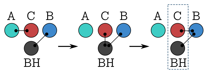
The picture above shows the process: Alice shares entanglement with Charlie, then throws her end into the black hole, which then radiates its end to Bob. So Charlie and the black hole should be maximally entangled with Bob.

The question is, how quickly does that happen? And Hayden and Preskill’s main result is that, after Bob collects $k + c$ qubits of new radiation, on average the reduced density matrix is close to maximally mixed, with the distance bounded by $2^{-c}$. “Average” here, I mean the Haar-avarage over the unitaries that the black hole could realise.

Generically, Charlie is entangled with both new and old radiation, so if you like, the original Bell pairs are distributed nonlocally throughout Bob’s system. In fact, Hayden and Preskill state that they don’t know if in general, the entanglement can be efficiently isolated. Kitaev and Yoshida show that it can (at least in the infinite temperature limit). If we wanted to perform some computations with Charlie, we would need to do this first.

You say “if the entanglement is there, why don’t we just project onto some conveniently defined entangled state?” Well, that’s exactly what the circuit does. But it takes work to define that canonical entangled state, and a bunch of pre-processing to ensure that projection is successful.

Technical preliminaries

Basics

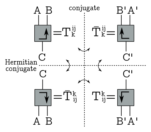
So, to build the circuit, we’re going to need some circuit building tools, aka tensor network jazz. As usual, a tensor is a box with some legs coming out, labelled by Hilbert spaces. A ket is a leg (or a bunch of legs) going up, while a bra is a bunch of legs going down (so time goes up in our diagrams). Flipping a tensor horizontally corresponds to taking complex conjugates, so the index structure is the same but the coefficients are conjugated; flipping it vertically is the Hermitan conjugate, so we conjugate coefficients and exchange upstairs and downstairs indices; and finally, rotating by $180^\circ$ is transposition, it just exchanges indices.

A dot on a line associated to a Hilbert space $B$ represents a normalisation factor $d_B^{-1/2}$. This will give us a quick way to write correctly normalised EPR pairs.

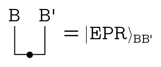
So we just take the identity, an unadorned line, bend one leg (taking us to $B’$ because we’ve transposed) and normalise it. In bra-ket notation what’s happening is:

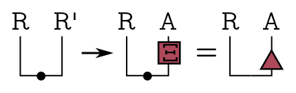
\[\frac{1}{d_B^{1/2}}\sum_i |i\rangle\langle i| \to \frac{1}{d_B^{1/2}} \sum_i |i\rangle |i^*\rangle.\]

Now, we could think of the Bell pairs shared by Alice and Charlie as just the EPR state on some system, but Kitaev and Yoshida consider the more general case that Alice has a big system $A$ and her share of the Bell pairs is embedded in that big system. There’s no secret information in that embedding, it’s just where she puts her entangled pairs in the larger system. Formally, we just set up the EPR state on Charlie’s reference system which we’ll call $R$, then embed Alice’s share in her big system $A$ using an isometry $\Xi: R’ \to A$. We lump these into a little triangle:

This has two legs pointing up, so we can think of as a pure state.

The black hole

So, what about the black hole? Let’s call the initial black hole system $B$, and we recall that its maximally entangled with a subsystem of the early radiation, which is isomorphic to $B’$. Here, we don’t keep track of the embedding in early radiation, we just focus on the subsystem $B’$.

So, we can represent the whole black hole evolution as follows.

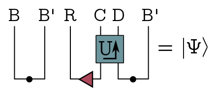
We start out with Alice and Charlie’s Bell pairs on the left, and the entangled black hole on the right. The black hole acts on $AB$ with some unitary operator $U$, then spits out some new Hawking radiation, which we’ll call system $D$, leaving some residual black hole degrees of freedom $C$. The result is just a big ket $|\Psi\rangle$ on $RCDB’$. Since $U$ is the most important box we’ll be using, I’ll just denote it with the arrow.

So, recall that the Hayden-Preskill protocol succeeds once there are no correlations between the remnant black hole $C$ and Charlie’s reference system $R$. All the entanglement is with Bob’s system. This means we want the reduced density $\rho_{RC}$ on $RC$ to be close to maximally mixed. The easiest way to measure this is the trace of the density squared, where $\mbox{Tr}[\rho^2_{RC}] \geq 1/d_Rd_C$, with equality just in case we have a maximally mixed density matrix. So an easy way to quantify how close to maximally mixed the system is by taking the trace squared, multiplying by the dimension and subtracting 1. We’ll call this little $\delta$:

\[\delta \equiv d_Rd_C\mbox{Tr}[\rho^2_{RC}] - 1 \geq 0.\]

The trace is the following diagram:

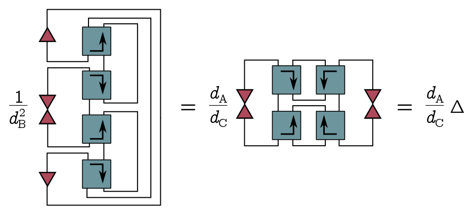
A density matrix will involve two boxes, so squaring it gives four. I’ve put the normalisation factors out the front for simplicity. Since this is just a number, I can fold this diagram in half without changing that number, and I get

If I add some dots, I can change the factor out the front from $1/d_B^2$ to $d_A/d_C$. We call the diagram with the dots big $\Delta$, and we can rewrite little $\delta$ as

\[\delta = d_A d_R\Delta - 1.\]

These deltas will be all important.

OTOCs

So far we haven’t said anything about the black hole evolution operator $U$, but for this whole business to work, we need to identify some properties of a typical random $U$ which will be useful for us. We’re going to assume that $U$ is perfectly scrambling, which loosely speaking, just means that out-of-time-order correlators (OTOCs) “factorise” in a nice way. Suppose we have operators $X$ and $Y$, which act on Alice’s system, and $W$ and $Z$, which act on the new radiation. All of these are defined at $t = 0$, so if we want to apply $W$ and $Z$ later in, we’re going to need to evolve them with $U$.

The definition of almost perfectly scrambling is that the OTOC we get from applying $X$ at time $0$, then $Z$ at a later time $t$, then $Y$ at $t = 0$, then $W$ at $t$ breaks into a sum of simpler expectations:

\[\langle W(t)Y(0)Z(t)X(0)\rangle \approx \langle WZ\rangle \langle Y\rangle \langle X\rangle + \langle W\rangle \langle Z\rangle \langle YX\rangle-\langle W\rangle \langle Z\rangle \langle X\rangle \langle Y\rangle.\]

For a maximally mixed state (which is what we start with) this is true for a randomly chosen $U$, in the sense that the Haar integral of the OTOC on the LHS equals the Haar integral of the RHS plus a term which is negligible when the Hilbert spaces involved are are large. Since the density matrix is uniform, we can write the OTOC as a trace:

\[\text{OTOC} = \frac{1}{d_Ad_B}\mbox{Tr}[U^\dagger WUYU^\dagger Z UX].\]

And of course, our favourite thing is to represent these traces diagramatically:

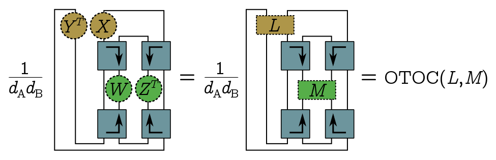
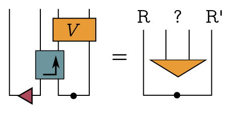
I’ve drawn the diagram to emphasize that the OTOC is actually a function of these composite objects, $\text{OTOC}(Y^T\otimes X, W \otimes Z^T)$. The virtue of doing things this way is that we can now extend the definition by linearity to arbitrary operators $L = \sum_j Y^T_j\otimes X_j$ and $M = \sum_k W_k\otimes Z_k$ acting on $A’A$ and $DD’$ respectively. This cute generalisation of the OTOC lets us write big $\Delta$ very simply as

\[\Delta = \text{OTOC}(L, M)\]

where $L$ involves some triangles, and $M$ is just the projector onto the EPR state in $DD’$:

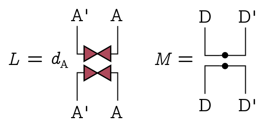
If $U$ is almost perfectly scrambling, we’re going to get an expression for $\Delta$, since that’s the the OTOC of $L$ and $M$ in this generalised sense. The RHS of the scrambling identity involves some traces of $X, Y$ (with similar statement for $W, Z$). Again, we can replace $Y^T \otimes X$ with $L$ and $W \otimes Z^T$ with $M$, and easily evaluate to find an upper bound on big $\Delta$, and hence on little $\delta$:

\[\begin{align} \frac{1}{d_Ad_R} & \leq \text{OTOC}(L, M) = \Delta \\ & \approx \frac{1}{d_A d_R} + \frac{1}{d_D^2} - \frac{1}{d_Ad_Rd_D^2} \\ & \leq \frac{1}{d_A d_R} + \frac{1}{d_D^2}\\ \quad \Longrightarrow \quad 0 & \leq \delta = d_Ad_R \Delta - 1 \leq \frac{d_Ad_R}{d_D^2}. \end{align}\]

The key point here is that if the black hole has this scrambling property, then we can make litte $\delta$ as small as we like by collecting enough Hawking radiation. To connect this back to Hayden and Preskill, if $d_A = d_R = 2^k$, and we collect $k + c$ qubits of Hawking radiation, so that $d_D = 2^{k+c}$, then

\[\delta \leq 2^{-2c}.\]

We only need to collect a few extra bits to make little $\delta$ tiny, and this will correspond to high fidelity recovery. I just want to point out that this story of almost perfect scrambling and OTOCs is much nicer, and more insightful, than Hayden and Preskill’s approach, where the black hole physics is hidden inside this thing called the decoupling inequality. Here, we can see what aspect of the physics is making things work.

Probabilistic decoder

With that mini-course on tensor networks out of the way, let’s talk about how to do the recovery. First of all, a perfect decoder is an operator that, from the big mess mess of entanglement in Bob’s system, cleanly isolates the EPR state with Charlie, which we can picture as follows:

In general, our decoder won’t be perfect, in the sense that it will only reproduce the EPR state up to some fidelity. That means you have a high probability of producing the EPR state if you perform a projective measurement onto it.

We warm up with the probabilistic decoder; we’ll improve this later by adding a Grover search phase to get a fully deterministic algorithm. But to start with, Bob’s going to get something maximally entangled with Charlie’s system, to high fidelity, but only with the miniscule probability $1/d_Ad_R$, which is exponentially small in the number of qubits involved. This is a bit like guessing what the message is, but if we guess right, we get something which is indeed maximally entangled with Charlie’s system, so that’s a successful decoding.

The basic idea is that Bob prepares a “guess” $|\xi_B\rangle$, which is just a copy of $|\xi\rangle$ living in copies of the systems $A’$ and $R’$: Remember that Bob has early radiation which is maximally entangled with the black hole. He can treat this as a copy of black hole, throw his guess into it and apply $U^*$.

That simulates the production of Hawking radiation! The final part of the algorithm projects the actual and fake radiation he’s collected onto the EPR state on $DD’$, which I drew as a triangle here.

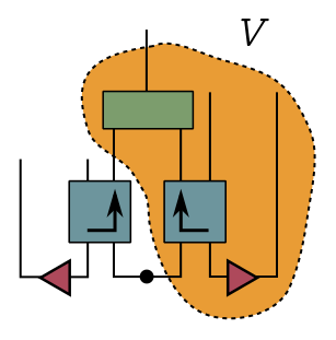
If that projection is successful, Bob gets the EPR state on Charlie’s system $R$ and his copy $R’$ with high fidelity. So he wins. If it’s unsuccessful, which is overwhelmingly likely, then Bob has to try again. Note that the area inside the dotted lines is the decoder.

So, let’s draw the system with both fake and real radiation, called $|\Psi_\text{in}\rangle$ since its the input to the radiation projector:

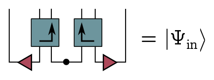
I want to draw your attention to the fact that this looks a lot like a wormhole. We have the real black hole on the left, a fake black hole on the right, and they are entangled. I’ll come back to this later.

The radiation projector $P_D = (|\text{EPR}\rangle_{DD’}{}_{DD’}\langle\text{EPR}|)\otimes I$ projects onto the EPR state on $DD’$ and does nothing the fake systems $C’$ and $R’$:

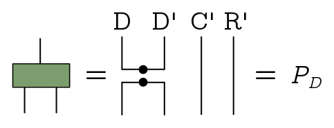
We can think of $P_D$ as part of a projective measurement consisting of ${P_D, I - P_D}$. Success is nonzero projection with $P_D$, and the probability that happens is the expectation of the operator. If we draw the diagram, you see immediately that the expectation is this number big $\Delta$ from earlier:

\[\langle\Psi_\text{in}|I_{RC}\otimes P_D|\Psi_\text{in}\rangle = \Delta.\]

Since $\Delta \geq 1/d_A d_R$, that’s our lower bound on the probability of successfully projection. So this is not a good lower bound.

If we do successfully project with the radiation projector $P_D$, then our chances of projecting onto the EPR state with Charlie are very good, the fidelity is high. And in fact, you can show that the fidelity (squared) is

\[F^2 = \frac{1}{1+\delta} \approx 1 - \delta.\]

So this is under control.

Deterministic decoder

Overview

So, our probabilistic decoder kind of sucks. The problem is this projection bottleneck, where we go from the input state $|\Psi_\text{in}\rangle$ to a target output state containing the EPR pair on $DD’$, but only with exponentially small probability. Once we do make it through this bottleneck, we’re good, we can reconstruct the state with high fidelity. What we would like to do is improve the probability of the radiation projection, and Kitaev and Yoshida propose to do that with quantum search. This is going to rotate our input vector $|\Psi_\text{in}\rangle$ to align* it with the target state.

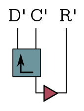
First, we define a projector $\tilde{P}_A$ onto Bob’s simulated black hole output:

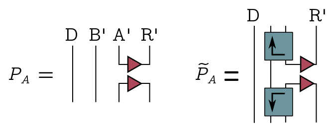
The operators we’ll use for the search algorithm are

\[W = 1 - 2P_D, \quad \tilde{W} = 2\tilde{P}_A - 1.\]

These look precisely like the “quantum oracle” and “Grover diffusion” operators in Grover search. The oracle function tells us when we have the right answer, it flips the sign when we act on the target state $|\text{EPR}\rangle_{DD’}$, and acts as the identity otherwise, and you can see this explicitly from the form of the operator. The diffusion operator $\tilde{W}$ on the other hand spreads amplitude around the space to aid in the search. The algorithm works by alternating between these operators some number of times, which gradually rotates the input vector.

Schmidt decomposition

When we run our search algorithm, we get a nontrivial product of projectors, $\Pi = \tilde{P}_AP_D\tilde{P}_A$:

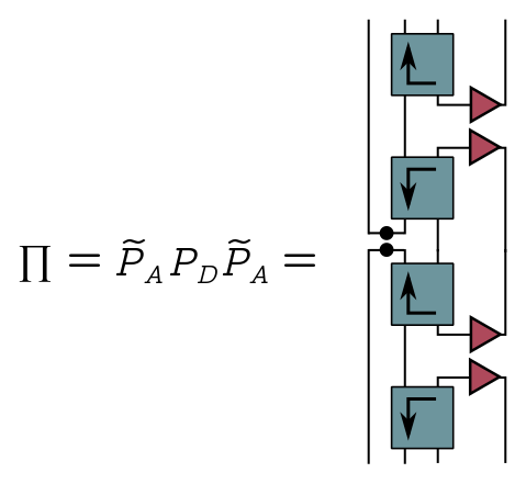
If we pull these operators in the middle to the left, we find that up to some constant, $\Pi$ is just the reduced density on Bob’s system:

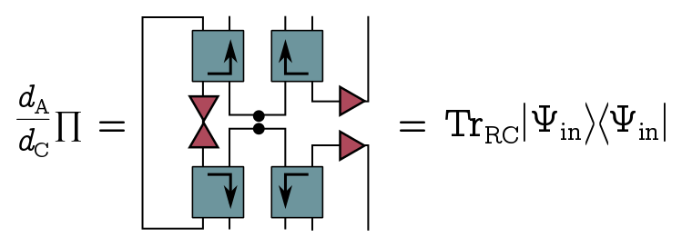
Our strategy will be to diagonalise this density and use Grover search on each eigenvector simultaneously. Let’s write the spectral decomposition of $\Pi$ (whatever it is):

\[\Pi = \sum_j \alpha_j |\psi_j\rangle\langle\psi_j|, \quad \alpha_j > 0.\]

To get the Schmidt decomposition of the input state $|\Psi_\text{in}\rangle$, we just tensor in some orthonormal vectors $|\eta_j\rangle$ on the complementary system $RC$:

\[|\Psi_\text{in}\rangle = \sum_j \sqrt{\frac{d_A}{d_C}}\sqrt{\alpha_j}|\Psi_j\rangle, \quad |\Psi_j\rangle \equiv |\eta_j\rangle\otimes|\psi_j\rangle.\]

Now we apply the radiation projector to each of the eigenstates:

\[|\Phi_j\rangle = \frac{I_{RC}\otimes P_D}{\sqrt{\alpha_j}}|\Psi_j\rangle.\]

I’ve inserted some factors to make sure it’s normalised. These are our target states, since they’re what we would get for each eigenvector $|\Psi_j\rangle$ if we successfully project. Applying the two projectors $\tilde{P}_A, P_D$, we find that $|\Phi_j\rangle$ and $|\Psi_j\rangle$ get mapped between themselves:

\[\begin{align*} I_{RC}\otimes P_D |\Psi_j\rangle & = \sqrt{\alpha_j}|\Phi_j\rangle, \quad I_{RC}\otimes P_D |\Phi_j\rangle = |\Phi_j\rangle \\ I_{RC}\otimes \tilde{P}_A|\Phi_j\rangle & = \sqrt{\alpha_j}|\Psi_j\rangle, \quad I_{RC}\otimes \tilde{P}_A|\Psi_j\rangle = |\Psi_j\rangle. \end{align*}\]

It follows that for each eigenindex $j$, the subspace $\mathcal{L}_j$ spanned by $|\Psi_j\rangle$ and $|\Phi_j\rangle$ is invariant under both projectors, and hence our search operators. Moreover, the subspace for different $j$ are orthogonal. So we just apply the search algorithm to each subspace simultaneously.

Grover search

There’s a nice way of thinking about what’s going on geometrically. We represent the $j$ subspace $\mathcal{L}_j$ on the plane, with $|\Phi_j\rangle$ in the $y$ direction and the orthogonal vector $|\Phi_j^\perp\rangle$ in the $x$ direction.

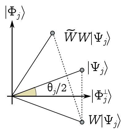
Define $\theta_j/2$ as the angle between the eigenvector $|\Psi_j\rangle$ and the $x$ axis. It’s easy to show that sin of this angle is just the square root of the eigenvalue, $\sin(\theta_j/2)= \sqrt{\alpha_j}$. Geometrically, the oracle operator $W = 1 - 2P_D$, is a reflection across the $x$ axis, while the diffusion operator $\tilde{W} = 2\tilde{P}_A - 1$ is a reflection across $|\Psi_j\rangle$. So acting with $W$ reflects us down here, and acting with $\tilde{W}$ brings us back up, having rotated anticlockwise by $\theta_j$. This is true for any vector, so each iteration of our search just rotates the vector anticlockwise by $\theta_j$.

We’re almost done, but to finish things off, we need to know more about these angles $\theta_j$, or equivalently, the eigenvalues $\alpha_j$. To begin with, let’s assume that they’re all the same. It’s not too hard to show that, in this case, they have to equal big $\Delta$, our probabability of successful projection in the first decoder, and $\Delta$ has to saturate its lower bound:

\[\alpha_j = \Delta=\frac{1}{d_Ad_R}.\]

In other words, this is the ideal case where $\delta = 0$. It follows that the initial angle is tiny, and from the small angle approximation,

\[\theta_j \approx \frac{2}{\sqrt{d_Ad_R}}.\]

So if we want to rotate our vectors to align* them as closely as possible to the target vectors, we iterate the search algorithm $m$ times, where

\[m = \frac{\pi}{2\theta_j} - \frac{1}{2} \approx \frac{\pi}{4}\sqrt{d_Ad_R}.\]

Then $m\theta_j \approx \pi/2$, so the vector will point in $y$ direction, which is what we want. Let’s assemble these rotated eigenstates into some big state $|\Psi(m)\rangle$. Whatever the eigenvectors are, by rotating, we’ve applied the same operator, namely the radiation projector $P_D$, to each of them. So our rotated vector $|\Psi(m)\rangle$ is exactly the state we wanted to project onto in the probabilistic decoder:

\[|\Psi(m)\rangle\approx \frac{1}{\sqrt{\Delta}}(I \otimes P_D)|\Psi_\text{in}\rangle.\]

We’re now done. At this point, we can recover the entangled state with Charlie, as we did before in the proabilistic decoder. And in fact, in this ideal case, we can do it with perfect fidelity since $\delta = 0$.

Of course, the angles may be different, but it turns out they can’t be too different. In the paper, the way they show is to forget about the angle themselves, and just bound the distance between the rotated vector $|\Psi(m)\rangle$, where the number of rotations is the same as before, and the target state $|\Psi_\text{out}\rangle$ with the EPR pair on the radiation. As it turns out, this distance is bounded above by something of the order $\sqrt{\delta}$:

\[\left|\left||\Psi(m^*)\rangle-|\Psi_\text{out}\rangle\right|\right| \leq \left(1+\frac{\pi}{2}\right)\sqrt{\delta}.\]

Putting it all together, we can reconstruct the EPR state with Charlie, with fidelity

\[F^2 = \langle\Psi(m^*)|P_R |\Psi(m^*) = 1 - \mathcal{O}(\delta).\]

And that’s the algorithm.

Conclusion

That pretty much wraps up the paper. I think there are a lot of neat ideas here, which remain to be exploited by the high energy community. In particular, it sharpens Hayden and Preskill’s story about the information-theoretic properties of scrambling, and connects them in an insightful way to the growing literature on chaos and OTOCs.

I wanted to end with a few comments. First of all, the paper is limited in that it doesn’t deal with thermal matrices (though this is rectified in the followup paper by Yao and Yoshida (2018) which I might discuss another time). Another proviso is that, in order for Bob to simulate the black hole, he needed to first isolate the EPR state on $BB’$ from the early radiation. As Hayden and Harlow (2013) showed in the heyday of firewalls, this is exponentially hard!

Here, Kitaev and Yoshida just black box that process. Since Bob is an asymptotic observer, he is not prevented from doing this (unlike Alice in Hayden and Harlow’s paper). But the point is that the real bottleneck for unscrambling is isolating the right subsystem of radiation, not finding the message in that subsystem.

Another problem is working out some sort of plausible dual geometry in the holographic context. Like I mentioned earlier, the input state $|\Psi_\text{in}\rangle$ is a lot like a wormhole. We have two black holes, one of them real and one of them simulated by Bob, and they’re entangled. The decoder actually lets you teleport gates from Charlie’s system $R$ to Bob’s copy $R’$ (exercise), which could be subsystems of entangled CFTs in the thermofield double. But we don’t have a perfect decoder, and to get a deterministic algorithm, we have to add the iterative search phase. We can express the search operators by iterating their generalised OTOC construction, so we would expect to get some sort of multiple shockwave geometry. On the gravity side, it’s not clear what this would buy us.