November 24, 2017. If I entangle two quantum computers, I sometimes get a wormhole, with each end associated to a computer. The amount of useful computation left on each system equals the volume of black hole spacetime left to safely jump into! “Safe” means you don’t get fried by a firewall or collide with junk thrown in from the other end of the wormhole. A summary of Uncomplexity and black hole geometry (Ying Zhao, 2017) for a group meeting.
Loosely speaking, uncomplexity is a measure of the amount of useful computation a quantum system can still perform. It is to computers what free energy is to thermodynamic systems. Zhao’s goal is to give an operational definition of uncomplexity when you only have access to part of the system. In this case, the part of the system we can access is in a mixed state.
 |
| A slightly more familiar computational resource. Source: Wikimedia Commons. |
For quantum information theorists, an operational notion of mixed-state uncomplexity might be useful, but I’m not sure what for. For holographers, though, Zhao gives a compelling gravitational interpretation when the quantum system is an asymptotically anti-De Sitter wormhole. In this case, the subsystem we control is one side of the wormhole. There is an older holographic story (reviewed below) suggesting that uncomplexity is dual to the volume of the black hole you can dive into, but Zhao goes further, identifying subregions dual to various interesting boundary operations. Let’s “dive into” the details!
Introduction
- Eternal black holes in Anti-de-Sitter (2001), Juan Maldacena.
- Fast Scramblers (2008), Yasuhiro Sekino and L. Susskind.
- The Complexity of Quantum States and Transformations: From Quantum Money to Black Holes (2016), Scott Aaronson.
- Quantum Complexity and Negative Curvature (2016), Adam R. Brown, Leonard Susskind, and Ying Zhao.
- The Second Law of Quantum Complexity (2017), Adam R. Brown and Leonard Susskind.
- a universal set of gates $\mathcal{G}$, i.e. a finite set we can use to build any unitary operator to desired precision; and
- a choice of precision $\epsilon$.
\mathcal{C}(U) \equiv \min \#\{\text{$\mathcal{G}$-circuits $\epsilon$-approximating } U\}. \]Morally speaking, we can define the complexity of a pure state $|\psi\rangle$ as the complexity of the unitary which prepares $|\psi\rangle$ from some reference state. If we are only interested in states connected by unitary time evolution, this naive definition works: the reference state is just the initial state $|\psi(0)\rangle$, and the unitary "preparing" the state at time $t$ is $U = e^{-iHt}$, so
\[
\mathcal{C}|\psi(t)\rangle = \mathcal{C}(e^{-iHt}).
\]This doesn't help us define the complexity of a mixed state. Typically, we care about mixed states that arise from tracing out a subsystem when the full state is pure, so we might think that we can just consider the state complexity of the purification. But we can get the same reduced density from different pure states, and in general, these pure states will have different complexities!
Fast scramblers and a second law
Now for some dynamics. Suppose you have $N$ qubits and want to build a quantum circuit model of a black hole. According to the standard lore black holes are fast scramblers, i.e. a local disturbance spreads exponentially and infects the whole system in the scrambling time $\tau_* \sim \log N$. There is a cute cartoon model of fast scramblers: the random circuit model, where we discretise time $\tau$, and at each time step, we choose a random element from our gate set $\mathcal{G}$ and a random subset of qubits for it to act on. Then we add this random gate it a chain of random gates. The near horizon region of the black hole performs computations approximately described by this circuit.So, at time $\tau$, we have a circuit $U(\tau)$ made of $\tau$ gates, and we can ask how its complexity $\mathcal{C}(\tau) \equiv \mathcal{C}[U(\tau)]$ changes with time. The current state of the art is numerology. The space of unitaries has dimension $\sim 4^N$, so an $\epsilon$-net spanning the space (which is specified by our approximation) has $\epsilon^{4^N} \sim e^{4^N}$ elements. It is large, and early on, the probability of "short circuits" (i.e. more efficient descriptions of the circuit) is basically zero. Thus, the complexity grows linearly, $C(\tau) \sim \tau$. Since the number of possible circuits grows exponentially with the number of gates, the maximum complexity is
\[
C_\text{max} \sim 4^N,
\] and hence the linear growth maxes out around $\tau \sim 4^N$. In the language of probability theory, adding random gates is a random walk in a high-dimensional circuit space. Initially, this space looks infinite, and hence non-recurring, to the walker; but walk long enough and you hit the boundary, where complexity starts to saturate. You can get recurrences which reset the complexity to near zero, but the Second Law of Quantum Complexity states that complexity almost always increases, or more precisely
If the complexity is less than maximum, it will most likely be in a local minimum.As the name suggests, there is a strong analogy between complexity and entropy. The big difference is that we have replaced combinatorics over states with combinatorics over operators. This means that the quantum complexity of a system with $N$ qubits behaves like the entropy of a classical system with $2^N$ degrees of freedom; this parallel can be made more precise using Nielsen's complexity geometry, which you can read about in Brown and Susskind's paper. Entropy can be expended uselessly, as when a gas expands in a box without a turbine; similarly, a black hole generates useless complexity, squandering its computational power on, well, simulating a black hole. Turning things around, in the same way that an entropy gap can be harnessed to deliberately move a system between macroscopic states, Brown and Susskind conjecture that a complexity gap can be harnessed to do quantum computations.
They give the concrete example of how adding a single "clean" qubit to a dirty old maxed out system allows to perform a useful computational task (in their example, computing a trace). Thus, we are led to define the uncomplexity
\[
\mathcal{UC}(\tau) \equiv \mathcal{C}_\text{max} - \mathcal{C}(\tau).
\]It should quantify the amount of useful computation the system can do.
Complexity = action, uncomplexity = interior
If the random circuit is a toy model for a black hole, what is the gravity dual of complexity?For illustrative purposes, suppose we have a one-sided AdS black hole, with an observer Alice stationed on the boundary. The proposed dual to complexity is the Einstein-Hilbert action of the Wheeler-deWitt (WDW) patch. The WDW patch consists of all spacelike surfaces anchored at boundary time $t$:
 |
| The (regulated) WDW patch for Alice. |
This proposed duality goes by the slogan "Complexity = Action". The action is of the same order as the volume $V(t)$, and a classical calculation shows that $V(t)$ does indeed grow linearly. For reasons I don't fully understand, at some late time $t_\text{cutoff}$, this classical linear growth stops, the black hole develops a firewall, and the interior spacetime breaks down. This defines a WDW patch of maximal complexity.
 |
| The maximal complexity patch. |
So, the uncomplexity (difference between the maximal WDW patch and Alice's current patch) is the volume of the blue patch in the following picture:
 |
| The interior spacetime available to Alice. |
But if Alice can ride along on the thin blue null line (e.g. encode herself into laser pulses), the blue patch is precisely the interior region of the black hole she can visit! So the uncomplexity is the interior spacetime available for Alice to visit when she hops into the black hole.
Uncomplexity for mixed states
With that preamble out of the way, let's finally start discussing the paper! As I said earlier, the idea of the paper is to define the uncomplexity of a mixed state in terms of the computational resources of a subsystem. In particular, we don't need to define the complexity of a mixed state; we do require some notion of pure state complexity however. Consider a bipartite system $AB$ in a pure state $|\psi\rangle_{AB}$, with reduced density matrices $\rho_A$ and $\rho_B$ belonging to Alice and Bob respectively. What sort of computations can Bob do with his density matrix? Well, Bob can apply unitaries $U_B$, and these generically increase the overall complexity of the state. So as a first try, we might think of the uncomplexity as the maximal increase in complexity of the state:\[
\mathcal{UC}(\rho_B) \overset{?}{\equiv} \max_{U_B}
\mathcal{C}(U_B|\psi\rangle) - \mathcal{C}|\psi\rangle.
\]But not every unitary is a useful computation for Bob. For instance, if Alice and Bob share a bunch of maximally entangled Bell pairs, then under a unitary $U_B$, Bob's density stays the same:
\[
\rho_B \to \rho_B \mapsto U^{\dagger}\rho_B U = \rho_B.
\]Bob's operation $U_B$ may perform computations, but the results are invisible to Bob. To capture useful computations, we subtract off the maximum complexity of these useless computations, rather than the current state complexity:
\[
\mathcal{UC}(\rho_B) \equiv \max_{U_B}
\mathcal{C}(U_B|\psi\rangle) - \max_{U_B^\dagger\rho_B{U_B} =
\rho_B}\mathcal{C}|\psi\rangle. \tag{1}
\]There is a neat way of thinking about this in terms of the Schmidt decomposition. In the Schmidt basis, $\rho_B$ is a diagonal matrix with $k$ distinct eigenvalues (including possibly zero):
\[
\rho_B = \lambda_i I_{N_1} \oplus \cdots \oplus \lambda_k I_{N_k} \oplus 0_{N_0}.
\]Call these components Schmidt blocks. Any "useless" computations $U_B$ by Bob that don't change $\rho_B$ are just separate rotations of the Schmidt blocks, or Schmidt rotations:
\[
U_B \in SU(N_1)\times \cdots\times SU(N_0).
\]These are precisely the unitaries that Alice can undo (by performing the inverse rotations). So we can also think of useful computations for Bob as those that Alice can't undo.
Black hole examples
A nice sanity check is the one-sided black hole (formed from a collapsing shell of photons), where the "subsystem" is in fact the whole system. We've already seen that, in this situation, uncomplexity can be interpreted as the volume of spacetime left for a boundary observer (now Bob rather than Alice) to jump into. We can interpret the terms of formula (1) geometrically: |
| Bob's uncomplexity for the one-sided black hole. |
Bob's only unitary is time evolution. He maximise complexity by evolving to the cutoff time
$t_\text{cutoff}$ (the first diagram), and the only way to leave his density matrix alone is to stay put (second diagram). The difference between the corresponding WDW patches in the interior
spacetime left for him to jump into.
The next example is the unperturbed two-sided black hole in AdS, dual to the thermofield double. The left side belongs to Alice and the right side belongs to Bob; we'll focus on Bob's subsystem. The idea here is that, if Bob's coarse-grained entropy is $S$, then he shares $S$ Bell pairs with Alice (they are involved in near-horizon computation):
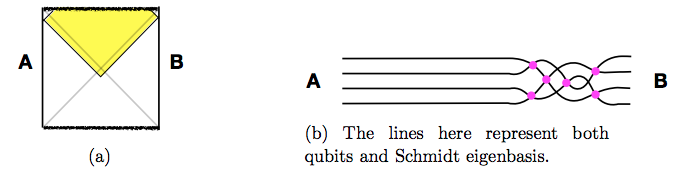 |
| Penrose and circuit pictures of the two-sided black hole. |
If they share $S$ Bell pairs, the density matrices are maximally mixed, and the uncomplexity is zero. Geometrically, Bob can go foward in time $t_R \to t_R + \Delta$, but Alice can go forward the same amount $t_L \to t_L + \Delta$ (where Alice's time goes down on the LHS) so that by boost symmetry, the WDW patch has the same size. Geometrically, we see that any change in complexity by Bob can be undone by Alice, which geometrically confirms that Bob has no uncomplexity.
But aren't we supposed to think of uncomplexity as interior spacetime? It seems like there is plenty of room in the wormhole. The lesson here (which will be made more precise below) is that uncomplexity is interior spacetime that you exclusively control. No one else can mess with it. So we might describe the wormhole as ER = EPR, and uncomplexity with the dorky slogan
\[
\mathcal{UC} = \text{U Control}.
\]
Perturbing the TFD
To understand things a bit better, let's perturb the thermofield double with a thermal photon, first on Alice's side and then on Bob's. Geometrically, if we throw in a photon, it gets seriously blueshifted and create a shockwave geometry, which tilts one side of the Penrose diagram. If we throw it in on Alice's side, she can still undo any operations by Bob by evolving an appropriate time forward. So Bob's uncomplexity is still zero.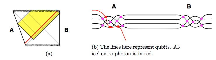 |
| Adding a thermal photon on Alice's side. |
What about if we give it to Bob instead? Since the thermal photon is the gravity dual of a single clean qubit, we expect it should buy Bob some uncomplexity. We can freely choose the left time (Bob can always undo that time evolution with his own unitary, as Alice could for him), so we can place it at a cutoff near the top of the Penrose diagram. The maximum complexity Bob can induce is given by some large cutoff time $t_R = t_\text{cutoff}$. If we throw in the photon at time $t_R = t_w$, we have to wait a scrambling time before the photon is incorporated into the quantum circuit. Before then, we can more or less ignore the perturbation, and the situation is basically the same as the two-sided black hole, with right time-evolution leaving Bob's density matrix unaffected. Thus, the second term in (1) is just given by the WDW patch anchored at whichever is bigger of the current time $t_R$, or the time when the photon is scrambled, $\max\{t_w+t_*, t_R\}$. Geometrically, we can picture the two possibilities as follows:
 |
| Correct uncomplexity equation for $t_R > t_w + t_*$. |
 |
| Not quite correct. |
This second diagram is not quite right because we ignored the thermal photon while it was scrambling. We will treat it more carefully in a moment! But the point is that the uncomplexity added to Bob's system is geometrically realised as a region inside the horizon that Bob exclusively controls, i.e. in his entanglement wedge.
Subregion duality
By now, we can see that computations changing Bob's density matrix are connected to the growth of his "one-sided black hole", that is, the interior spacetime in his entanglement wedge. So we would expect the computations which don't change his density matrix, i.e. the Schmidt rotations, fuel the growth of the entanglement region between Alice and Bob. Thus, there is a subregion duality connecting types of operations to regions of space. To check this, it's possible to do a more precise matching between the volume growth of different regions as the photon gets scrambled, creating an "epidemic" of "sick" gates in the quantum circuit.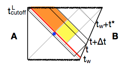 |
| Different regions store different gates. |
Up to some minor technical differences, the growth of the entanglement region (orange) matches the operations that can still be undone by Alice, i.e. healthy gates, while the the growth of Bob's entanglement wedge (yellow) matches the number of sick gates. In some sense, the Schmidt rotations are "stored" in the orange entanglement region, while Bob's useful (detectable) computations are
stored in the yellow region.
This lets us draw the correct geometries for uncomplexity while the photon is being scrambled. We have to redraw the second diagram slightly in our earlier picture:
 |
| Correct for $t_w < t_R < t_w+ t_*$. |
Basically, we leave the operations in the entanglement region alone since this where Schmidt rotations are stored, and shouldn't be affected by the scrambling of the photon. However, within Bob's entanglement wedge, the epidemic growth leads to operations that cannot be undone by Alice; hence can be detected by Bob; and hence do not contribute to computations which don't change Bob's density matix. So we have to excise part of the patch in Bob's entanglement wedge beyond the null line emanating from $t_R$.