Entanglement and quantum secrecy
June 16, 2017. A presentation for the Melbourne Maths and Science Meetup on entanglement and quantum key distribution. Although the talk was pitched at a general audience, the notes here are more technical.
Table of Contents
1. Quantum Mechanics
We’re going to start our journey towards entanglement with the famous experiment of Stern and Gerlach. From there, we can motivate the basic ideas of quantum mechanics with a liberal dose of hindsight and handwaving.
1.1. Stern-Gerlach and Quantisation
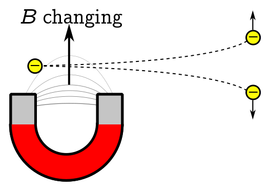
Particles in atoms — electrons, protons, and neutrons — contain an intrinsic dipole moment or spin, essentially a little bar magnet attached to the particle. This means that — independent of their charge — these particles are deflected by changing magnetic fields. In an atom, spins like to pair up and cancel out, since this is a lower energy state. Thus, there exist atoms (most importantly silver) which are electrically neutral, with a single unpaired electron left over; their response to a magnetic field is effectively determined by a single electron spin.
In the Stern-Gerlach (SG) experiment, we shoot a whole bunch of silver atoms through a magnetic field, with a photographic plate at the other end to register the trajectory of the atoms. Suppose the magnetic field is changing in the $z$ direction. If the atoms move through the apparatus quickly enough, the deflection is simply proportional to $z$ component of their spin. We expect the spins to be randomly oriented, since we haven’t done anything to align them, so they should produce a continuous distribution on our photographic plate. What actually happens is extremely surprising! Instead of a continuous distribution, we get two sharp peaks of equal strength, corresponding to spins in the $\pm z$ direction:
This is bizarre. The peaks can only be explained by supposing that the randomly oriented spins snap (with equal probability) to the $\pm z$ directions when they pass through the field. There are two more relevant experimental facts. First, if we apply another SG apparatus to either the up or the down spins separately, nothing happens: we observe a single peak corresponding to the spin we selected. Second, if we rotate the second SG apparatus by $90 ^\circ$ (say the field changes in the $x$ direction), we get the same “spin snapping” effect, with a new bimodal distribution along the $x$-axis.
1.2. Quantum Mechanics = Linear Algebra
Our original SG apparatus is designed to measure the component of spin in the $z$ direction. Classically, if there is no $z$ component, there is no deflection. We find, however, that the outcome of this measurement is quantised: we can only get spin up or spin down in the direction of the field. Making sense of this experiment required the greatest revolution in scientific thought since Isaac Newton. Rather than recapitulate this convoluted history, we’re going to skip ahead to the answer and check that it works. However, see 1.4 for more on the history of quantum mechanics.
For simplicity, we focus on the unpaired electron in the silver atom. In the SG experiment, only the spin up and spin down states show up. Thus, we hypothesise that the spin of the electron is not a spatial vector with some fixed orientation, but instead a linear combination (a sum with coefficients) of the two states that matter, spin up and spin down. We denote vectors as labels surrounded by funny brackets, “$|\text{label}\rangle$”. Using this notation, we call the spin state $|\psi\rangle$, and the special spin up and spin down states $|0\rangle$ and $|1\rangle$ respectively. Our hypothesis means we can write $|\psi\rangle$ explicitly as a combination of spin states, or implicitly as a column vector:
\[|\psi\rangle = \alpha|0\rangle + \beta|1\rangle \equiv \left[\begin{array}{c} \alpha \\ \beta \end{array}\right].\]It turns out that we need to make $\alpha$ and $\beta$ complex numbers; I will explain why below. Let’s call the two-dimensional vector space of these linear combinations $V_2$.
What does a measurement do to these vectors? First of all, measurements produce numbers. In the case of the SG apparatus, we can think of it as giving $\pm 1$ depending on whether it sees a spin up ($+1$) or a spin down ($-1$). And, if $|\psi\rangle$ happens to equal spin up or spin down, it leaves it alone, as the second SG apparatus shows. There is a nice way to integrate these different facts, but before we do that, let me remind you of some linear algebra. A linear transformation on $V$ is a function $A: V \to V$ with the property that
\[A(\alpha|\psi\rangle + \beta|\phi\rangle) = \alpha A|\psi\rangle + \beta A|\phi\rangle\]for any vectors $|\psi\rangle, |\phi\rangle \in V$ and complex numbers $\alpha, \beta \in \mathbb{C}$. Equivalently, we can write $A$ as a matrix
\[A = \left[\begin{array}{cc}A_{00}&A_{10}\\A_{01}&A_{11}\end{array}\right],\]and figure out $A|\psi\rangle$ using matrix multiplication. It is also helpful to note that the columns of $A$ are just the image of the basis vectors $|0\rangle, |1\rangle$,
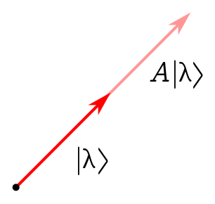
\[A|0\rangle = \left[\begin{array}{c} A_{00} \\ A_{01} \end{array}\right], \quad A|1\rangle = \left[\begin{array}{c} A_{10} \\ A_{11} \end{array}\right].\]Finally, an eigenvector $|\lambda\rangle$ of $A$ is a vector which $A$ streteches by a factor $\lambda$, the corresponding eigenvalue:
\[A|\lambda\rangle = \lambda|\lambda\rangle.\]We illustrate this below:
Phew! With all that linear algebra out of the way, we can finally outline the quantum mechanical version of what’s happening in the SG experiment. Having hypothesised that spin states are vectors in $V_2$, we now suppose that the SG apparatus acts as a linear operator on $V_2$. We’ll call this operator $Z$, since we measure the spin in the $z$-direction. Furthermore, we suppose that the eigenvectors of $Z$ are the spin up and spin down states, with eigenvalues respectively $\pm 1$. This immediately implies that $Z$ is given by
\[Z = \left[\begin{array}{cc}1&0\\0&-1\end{array}\right].\]Let’s restate our conclusions once more:
Measurement corresponds to a linear operator acting on a vector space of states $V$. Eigenvectors of the operator return their eigenvalues as measurement results. If the spin state is an eigenvector, it does not change after measurement.
This is all well and good, but what about states that are not eigenvectors? We’ll consider this in the next section.
- Exercise 1.1. Confirm that $Z$ has the eigenproperties $Z|0\rangle = 1$ and $Z|1\rangle = -1$.
- Exercise 1.2. Consider the matrices
Find the eigenctors and eigenvalues. (As the notation suggests, $X$ and $Y$ correspond to measuring the spin in the $x$- and $y$-direction, so you can anticipate eigenvalues $\pm 1$.)
1.3. Intrinsic Randomness
We have yet to explain why randomly oriented spin states “snap” into the special spin up and spin down states. At this point, the weirdness of quantum mechanics truly rears its head. Suppose we have a spin state1
\[|\psi\rangle = \left[\begin{array}{c} \alpha \\ \beta \end{array}\right], \quad |\alpha|^2 + |\beta|^2 > 0.\]To explain the mechanics of “snapping”, we make a bold hypothesis: our state $|\psi\rangle$ snaps to the spin up or spin down state randomly, with probabilities given by
\[\begin{align*} p_0 & \equiv p(|0\rangle \text{ after measurement}) = \frac{|\alpha|^2}{|\alpha|^2 + |\beta|^2} \\ p_1 & \equiv p(|1\rangle \text{ after measurement}) = \frac{|\beta|^2}{|\alpha|^2 + |\beta|^2}. \end{align*}\]For a random distribution of coefficients $\alpha, \beta$, from symmetry we would expect that half the time the spins snap to spin up, and half the time they snap to spin down. 2
Classical physics is a set of deterministic, clockwork theories. Even in situations which necessitate the use of probability (e.g. thermodynamics), we are modelling our ignorance, and assume that at a basic level, physical objects are still behaving in a definite way. Quantum mechanics is such a huge conceptual shift because it posits basic, unavoidable randomness in nature.
As a quick sanity check, we see that $p_0 + p_1 = 1$. We also note that rescaling $\alpha$ and $\beta$ by a common factor so that the numerator of these expressions equals $1$ does not change the probabilities. (Equivalently, we are just rescaling the whole vector.) It turns out3 this rescaling doesn’t affect anything else, so from now on we assume
\[|\alpha|^2 + |\beta|^2 = 1.\]There is a more elegant way to extract the probabilities $p_0, p_1$ using an inner product. First, we denote the Hermitian conjugate of a complex matrix $A = [A_{ij}]$ by
\[A^\dagger = [A_{ij}]^\dagger = [A^*_{ji}].\]In other words, we swap rows and columns and complex conjugate all the entries. The inner product of two complex vectors is
\[\left[\begin{array}{c} \alpha_1 \\ \beta_1 \end{array}\right] \cdot \left[\begin{array}{c} \alpha_2 \\ \beta_2 \end{array}\right] = \left[\begin{array}{c} \alpha_1 \\ \beta_1 \end{array}\right]^\dagger \left[\begin{array}{c} \alpha_2 \\ \beta_2 \end{array}\right] = \left[\begin{array}{cc} \alpha_1^* & \beta_1^* \end{array}\right] \left[\begin{array}{c} \alpha_2 \\ \beta_2 \end{array}\right] = \alpha_1^*\alpha_2 + \beta_1^*\beta_2.\]More abstractly, if $|\psi\rangle$ is a vector, we denote $|\psi\rangle^\dagger = \langle \psi|$, and $|\psi\rangle \cdot |\phi\rangle = \langle \psi |\phi\rangle$. We also note that our inner product is “conjugate symmetric” and linear in the second argument:
\[\langle \psi | \phi\rangle = \langle \phi | \psi\rangle^*, \quad \langle \psi| (\alpha|\phi\rangle + \beta|\xi\rangle) = \alpha\langle \psi |\phi\rangle + \beta\langle \psi|\xi\rangle.\]It also follows from our normalisation of coefficients that every vector has unit inner product with itself:
\[|\psi|^2 \equiv \langle\psi |\psi\rangle = |\alpha|^2 + |\beta|^2 = 1.\]We call $|\psi|$ the norm of the vector, so every state has unit norm. Finally, here is our elegant expression for the probabilities:
\[p_n = |\langle \psi | n \rangle|^2, \quad n = 0, 1.\]The complex numbers $\alpha = \langle \psi | 0 \rangle$, $\beta = \langle \psi | 1 \rangle$ are called amplitudes. If the spin snapped to state $|n\rangle$, the measurement yielded the corresponding eigenvalue $(-1)^n$. This leads to another quantum mechanical dictum:
After measuring a state $|\psi\rangle$ it snaps to eigenvector $|n\rangle$ of the measurement operator with probability $|\langle\psi|n\rangle|^2$, and yields the corresponding eigenvalue $\lambda_n$.
What I’ve called “snapping” is more conventionally (and melodramatically) called “collapse”.
- Exercise 1.3. Show that $|0\rangle$ (spin up in the $z$-direction) snaps with probability $1/2$ to spin up or spin down in the $x$-direction. This explains why applying a second SG apparatus to the spin up particles, oriented in the $x$-direction, produces a new bimodal pattern.
- Exercise 1.4. Prove that the inner product is conjugate symmetric and linear in the second argument.
1.4. The Schrödinger equation
We still have a few loose ends to tie up before we move on to entanglement. First of all, why do we use complex numbers? Couldn’t we forget about amplitudes altogether, and just use probabilities? And even if we do use amplitudes, why do they have to be complex? The short answer is the Schrödinger equation. If $H$ is the operator measuring energy, then an arbitrary state $|\psi\rangle$ evolves in time according to the differential equation4
\[i \frac{\partial |\psi\rangle}{\partial t} = H |\psi\rangle.\]This has nothing to do with measurement or collapse; this describes evolution between measurements. The appearance of $i = \sqrt{-1}$ is a sign that quantum mechanics must involve complex numbers. Even if we start off with real linear combinations of vectors, the evolution turns them into complex linear combinations! I’ll conclude the section with a few optional snippets.
1.4.1. *Making Light of the Schrödinger equation
Light can be thought of a sinusoidal wiggle moving through space at $c = 3\times 10^8$ m/s. The top of wiggle is called a crest. The frequency of the wave is the number of crests passing a given spot per second, while the wavelength is the distance between adjacent crests.
In 1905, Einstein explained the photoelectric effect5 by positing that light is made of quanta, discrete packets of energy. The lump of energy in each quantum is related to the frequency by
\[E = 2\pi f \equiv \omega,\]where $\omega$ is the angular frequency. It’s not hard to show that the speed of the wave is the product of wavelength and frequency, so
\[c = f\lambda \equiv \frac{\omega}{k}, \quad k \equiv \frac{2\pi}{\lambda}.\]A simple equation for a sinusoidal wiggle is
\[g(x, t) \equiv \cos\left(kx - \omega t\right).\]As you can check, this satisfies a wave equation
\[\frac{\partial^2 g}{\partial x^2} = \frac{1}{c^2}\frac{\partial^2 g}{\partial t^2}.\]However, if you shift the cosine term you get a sine term. Multiply it by $i$, add them together, and use Euler’s formula:
\[h(x, t) \equiv \cos\left(kx - \omega t\right) + i \sin\left(kx - \omega t\right) = e^{i(kx - \omega t)}.\]Since this is just a sum of waves moving at speed $c$, it certainly obeys the wave equation, but in fact, it satisfies an even simpler equation:
\[i\frac{\partial h}{\partial t} = \omega h = Eh,\]remembering Einstein’s identification $E = \omega$. This is pretty much the Schrödinger equation. Schrödinger first wrote down the equation while on vacation in the Swiss Alps in 1925. The big step was to apply this to everything and not just light. Schrödinger was convinced that everything should satisfy a wave equation by the work of de Broglie on matter waves in 1924.
1.4.2. *Ghosts and Hermits
It just so happens that for our spin observable $Z$, there are two eigenvectors with real eigenvalues. If we had a matrix with fewer eigenvectors, we can run into a serious problem: the transition probabilities don’t add up to 1! Another problem is that eigenvalues (allowed measurement outcomes) could be imaginary. If you ask how big something is, and you get the answer “$i$”, something has probably gone wrong.
We can solve these problems in one fell swoop by insisting that measurements correspond to operators which equal their own Hermitian conjugate. More simply, these are called Hermitian operators:
\[A^\dagger = A \quad \text{ or equivalently } \quad A_{ij}^* = A_{ji}.\]Why? First of all, this guarantees that the eigenvectors are real. Suppose that $A|\lambda\rangle = \lambda|\lambda\rangle$. Then, since $\langle \lambda |\lambda\rangle = 1$,
\[\lambda = \langle \lambda | (\lambda|\lambda\rangle) = \langle \lambda | (A |\lambda\rangle) = |\lambda\rangle^\dagger A |\lambda\rangle = |\lambda\rangle^\dagger A^\dagger |\lambda\rangle = (A|\lambda\rangle)^\dagger |\lambda\rangle = \lambda^*.\]This means $\lambda$ is a real number! A second reason for restricting to Hermitian operators is a powerful mathematical result called the spectral theorem. This guarantees that, for any Hermitian matrix $A$, the eigenvectors of $A$ form an orthonormal basis for the space $V$:
\[A|n\rangle = \lambda_n |n\rangle, \quad \langle m | n\rangle = \delta_{mn}, \quad \text{span}(|1\rangle, \ldots, |d\rangle) = V.\]This can be extended with a little care to infinite-dimensional spaces (needed for standard treatments of quantum mechanics), but we will deal exclusively with finite-dimensional spaces in these notes.
It is an axiom of quantum mechanics that any genuine measurement we can make corresponds to some Hermitian operator. Conversely, any Hermitian operator should correspond to some measurement. However, experimentally realising operators can be an extremely tricky business, a point we will return to later.
- Exercise 1.5. Verify that $X, Y$ and $Z$ are Hermitian, and satisfy the spectral theorem.
- Exercise 1.6. Let $V_d$ be a vector space of dimension $d$, and $A$ a Hermitian operator with orthogonal eigenvectors $|n\rangle, n = 1, \ldots, d$. Prove that, for any unit-norm $|\psi\rangle \in V_d$, the transition probabilities add to $1$.
1.4.3. *Spin States Live on a Sphere
Recall that we started with a vector space $V_2$, consisting of all linear combinations of the form
\[\alpha|0\rangle + \beta|1\rangle, \quad \alpha, \beta \in \mathbb{C}.\]Thus, to begin with we have two completely unconstrained complex parameters, or $2\times 2 = 4$ real parameters, since each complex number encodes two real numbers, $\alpha = \alpha_1 + i\alpha_2$. We then argued that we could rescale physical states (other than the zero vector), which represents a single complex constraint, or two real constraints. Alternatively, we fix $|\alpha|^2+|\beta|^2 = 1$ and identify unit norm states which differ only by a phase $e^{i\theta}$. Either way, we only have two real parameters.
What does the overall space look like? There is a nice way to visualise it which also has applications in quantum computing. Since $|\alpha|^2 + |\beta|^2 = 1$, we can identify
\[|\alpha| = \cos\left(\frac{\theta}{2}\right), \quad |\beta| = \sin\left(\frac{\theta}{2}\right), \quad 0 \leq \theta \leq \pi,\]where we restrict $0 \leq \theta \leq \pi$ so that both sine and cosine are positive. We can always multiply by a total phase factor so that $\alpha$ is real, and $\beta = e^{i\phi}|\beta|$ for $0 \leq \phi \leq 2\pi$. We also note that $\phi$ is periodic, since $e^{2\pi i} = e^0 = 1$. Assembling these two facts, we see that the space of spin states looks like a sphere, called the Bloch sphere:
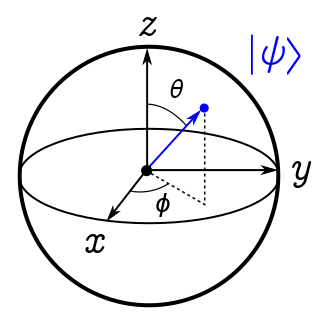
Just to be explicit, the map from the Bloch spherical coordinates $(\theta, \phi)$ to spin states is given by
\[|\psi(\theta, \phi)\rangle = \cos\left(\frac{\theta}{2}\right)|0\rangle + e^{i\phi}\sin\left(\frac{\theta}{2}\right)|1\rangle = \left[\begin{array}{c} \cos\left(\theta/2\right) \\ e^{i\phi}\sin\left(\theta/2\right) \end{array}\right].\]We can relate the geometry of the sphere to the eigenstates of spin in the $x$-, $y$- and $z$-directions, as the exercise below shows.
- Exercise 1.7. Show that eigenvectors of $X$ (respectively $Y$) are in the $\pm x$ ($\pm y$) directions, as shown in the diagram.
2. Entanglement and Computation
So far, we have been discussing the spin of a single electron; according to quantum mechanics, this must be modelled as a state living in a vector space $V_2$. Entanglement is a relation between systems, so we have to figure out what happens when we put two systems together.
2.1. Glomming Quantum Systems
In general, quantum mechanical systems are vector spaces. Thus, we need to think about how to join two vector spaces $U, V$ together to form a new vector space $W$. One way to approach is to constrain the joining of systems at the level of a joining operation $\otimes : U \times V \to W$, which takes individual vectors in $U$ and $V$ and returns a vector in $W$:
\[|u\rangle \in U, |v\rangle \in V \mapsto |u\rangle \otimes |v\rangle \in W.\]What properties should this joining operation have? Most importantly, we want glomming to respect the structure of each vector space. This means switching back and forth between the combined systems and the individual systems won’t mess up the algebra. Put another way, if the second system is in some fixed state $|v\rangle$ (it could be an unconnected spin on the other side of the universe), we need to be able to manipulate the first system independently. Mathematically,
\[(\alpha|u_1\rangle + \beta |u_2\rangle)\otimes |v\rangle = \alpha|u_1\rangle\otimes |v\rangle + \beta |u_2\rangle\otimes |v\rangle,\]with a similar relationship for linear combinations in the second argument. We call such an operation bilinear.
Our second requirement is that $W$ contain copies of $U$ and $V$. For instance, fixing $|v\rangle \in V$ and using linearity in the first argument, we get
\[\left(\sum_{k=1}^{\text{dim } U}\alpha_k|u_k\rangle\right)\otimes |v\rangle = \sum_{k=1}^{\text{dim } U}\alpha_k|u_k\rangle\otimes |v\rangle \in W,\]where $|u_k\rangle$ is a basis of $V$. As long as the $|u_k\rangle \otimes |v\rangle$ are linearly independent (no linear combination of them vanishes), this embeds a copy of $U$ in $W$.
A minimal way to ensure this is to define $W$ as a new space with basis vectors
\[|w_{ij}\rangle \equiv |u_i\rangle \otimes |v_j\rangle, \quad 1 \leq i \leq \text{dim } U, \quad 1 \leq j \leq \text{dim } V,\]where in addition, $\otimes$ is bilinear. This is called the tensor product, since bilinearity looks very much like the distributivity property of the humdrum product of scalars. In other words, the glommed system $W$ has dimenion $\text{dim } U \cdot \text{dim }V$. You can check this ensures the independence condition above. The operation $\otimes$ applies to individual vectors, but also tells us how to glom the systems $U$ and $V$, so we can write $W = U \otimes V$.
- Exercise 2.1. Show that $\otimes$ as defined above embeds copies of $U$ and $V$ in $W$.
2.1.1. *Direct sums
If you have some linear algebra, you might wonder why we don’t use the direct sum $\oplus$ instead. This obeys the rule
\[(\alpha_1|u_1\rangle + \alpha_2|u_2\rangle) \oplus (\beta_1|v_1\rangle + \beta_2|v_2\rangle) = (\alpha_1 |u_1\rangle \oplus \beta_1 |v_1\rangle) + (\alpha_2 |u_2\rangle \oplus \beta_2 |v_2\rangle).\](Equivalently, we can put $|u\rangle$ and $|v\rangle$ into a big column vector $[|u\rangle, |v\rangle]^T$ and add in the usual way.) This is the wrong rule for glomming systems, since we cannot generally fix the state of, say, the second system and do linear algebra in the first. In fact, the direct sum is only linear in one argument when the fixed argument is the zero vector! As we discovered earlier, this is not even a physical state.
Another way of seeing the problem is to look at basis vectors, which encode the basic physical states of the system (e.g spin up and spin down for $V_2$). For the direct sum $U \oplus V$, we can cobble together a basis from the bases of $U$ and $V$:
\[\{|u_1\rangle, \ldots, |u_{\text{dim }U}\rangle, |v_1\rangle, \ldots, |v_{\text{dim }V}\rangle\}.\]Thus, glomming with $\oplus$ implies that the basic states of the combined system are the states of $U$ or the states of $V$. In particular, the combined system could be in some basic physical state of $U$ (e.g spin up for $U = V_2$) but have no information about the second system. This makes no sense! We have to specify what’s going on in both systems, which is precisely what the basis of the tensor product ${|u_i\rangle\otimes|v_j\rangle}$ captures.
2.2. Entanglement defined
Now we know how to put quantum systems together, let’s consider the simplest composite system: two electron spins, $V_2^2 \equiv V_2\otimes V_2$. This has basis vectors
\[|0\rangle\otimes |0\rangle \equiv |00\rangle, \quad |0\rangle\otimes |1\rangle \equiv |01\rangle, \quad |1\rangle\otimes |0\rangle \equiv |10\rangle, \quad |1\rangle\otimes |0\rangle \equiv |11\rangle.\]Our basis vectors are nicely labelled by a string of two binary digits, or a binary $2$-string. (We can do the same trick for $n$ glommed copies of $V_2$, yielding a vector space $V_{2}^n$ with basis vectors labelled by the $2^n$ binary $n$-strings.)
Now, since $V_2^2$ is a vector space, the physical “two-spin” states are just any normalised vectors,
\[|\psi\rangle= \sum_{i,j=0}^1 \alpha_{ij} |ij\rangle = \alpha_{00}|00\rangle+\alpha_{01}|01\rangle+\alpha_{10}|10\rangle+\alpha_{11}|11\rangle, \quad \sum_{i,j=0}^1 |\alpha_{ij}|^2 = 1.\]A two-spin state $|\psi\rangle$ can either:
- factorise into tensor product of two single spin states; or
- fail to factorise into single spin states.
The two-spin states which factorise are called separable, while the second type are called entangled. Entanglement is the failure of a state to factorise across a tensor product of vector spaces!
We will see some of the remarkable operational consequences soon, but before that, let’s look at some example. Any of the basis states of $V_2\otimes V_2$ are separable, e.g. $|01\rangle$. However, there are more interesting separable states like
\[\frac{1}{\sqrt{2}}(|0\rangle+|1\rangle)\otimes \frac{1}{\sqrt{2}} (|0\rangle+|1\rangle) = \frac{1}{2}(|00\rangle + |01\rangle + |10\rangle + |11\rangle).\]For entangled states, how do we check that no tensor product of single spin states works? Well, consider an arbitrary separable state,
\[(\alpha|0\rangle+\beta|1\rangle)\otimes (\gamma|0\rangle + \delta \alpha|1\rangle) = \alpha\gamma|00\rangle + \alpha\delta|01\rangle + \beta\gamma|10\rangle + \beta\delta|11\rangle.\]Let’s label the coefficients using $\alpha_{ij}$ as above. Apart from the usual normalisation $|\alpha|^2+|\beta|^2 = |\gamma|^2 + |\delta|^2 = 1$, we can see the coefficients are related by
\[\alpha_{00}\alpha_{11} = \alpha_{01}\alpha_{10} = \alpha\beta\gamma\delta.\]Turning it round, if this condition holds, we can always find $\alpha, \beta, \gamma, \delta$ satisfying the constraints, and the state is separable.
2.3. Spooky action
So, if Alice and Bob share an EPR pair, and they measure their qubits in any order, when they later compares notes they find they always measure opposite states. The qubits knows about each other instantaneously — even though Bob and Alice are on opposite sides of the galaxy. Einstein and co called this “spooky action at a distance”, and concluded that quantum mechanics couldn’t be the whole story.
Experimentally speaking, we now know that entanglement is a real thing, but let’s see what freaked Einstein out. For EPR, the deal-breaker was the violation of a fundamental physical principle called locality: roughly, the idea that you can only physically influence nearby things. There’s a very strong reason to love, honour and obey locality, connected to special relativity. If we can transmit information faster than the speed of light, then you can easily build a time machine which sends information backwards in time (illustrated below). All you need to do is arrange the receivers to be moving relative to each other. This gives rise to all the paradoxes of time travel.
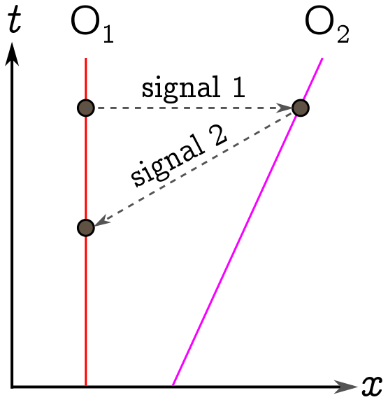
Two observers, $O_1$ and $O_2$, build a time machine by transmitting signals instantaneously (in their reference frames). Signal 1 is instantaneous in the frame of $O_1$, while signal 2 is instaneous in the frame of $O_2$. This means $O_1$ receives the signal in the past!
But since entanglement is a non-local, instantaneous connection between Alice and Bob’s qubits, it seems they can make a time machine! All Alice needs to do is jerry-rig the system so her qubit goes into particular states. Bob then measures his system, flips the bits, and has a message encoded in binary.
Luckily for the space-time continuum, Alice can’t jerry-rig the system this way. Quantum mechanics got us into this mess, and it saves us; although it permits entanglement, it prevents Alice from shoehorning a qubit into a desired state. The outcome of her measurements is always random, always out of her control. Bob may learn that outcome instantaneously, but because it can’t be controlled, it can’t be used to transmit information. The moral of the story is that entanglement really is spooky and non-local. But it respects a weaker property called causality: no faster than light messaging, and hence, no time machines.
3. Quantum Key Distribution
3.1. Introduction
But although we can’t use entanglement to send information, Alice and Bob share a resource — the value of the measurement — without having to communicate about it classically. This shared resource can be used for quantum key distribution (QKD). The goal for Alice and Bob is to share a string of random bits, over an unsecure channel, and check that it hasn’t been snooped on. They can then use the random string as a parameter for encrypting subsequent messages. It doesn’t matter that the key is random — all that matters is that they share the key and nobody else does. Let’s call the adversary Eve. Her goal is to figure out Alice and Bob’s shared key without them realising. Otherwise, even if Eve knows the key, they won’t use it!
3.2. One basis
Let’s start with a simple scheme that doesn’t work. We suppose that Alice and Bob have an infinite source of EPR pairs, which sends one qubit to Alice, and another to Bob. They can generate as many of these pairs as they like. Alice and Bob make measurements on each pair as it comes in. Since the qubits are entangled, they will get opposite results. They can generate a string of bits — as long as they like — by simply making Alice’s measurements the shared string. All Bob needs to do is flip his bits to obtain precisely the same bit string as Alice.
The problem is that there is no way for them to guard against Eve. For instance, suppose Eve measures Alice’s qubit en route. If Eve observes a $|0\rangle$, the EPR pair becomes a product state:
\[|\text{EPR}\rangle \to |0\rangle|1\rangle.\]Now Alice will measure $0$, and Bob will measure $1$. They will still be able to construct a shared bit string, but Eve will know it as well. Note that Eve’s measurement destroys the entanglement between Alice and Bob’s qubit. This gives us a clue about how to detect interference: we need a scheme where the loss of entanglement, before the qubits arrive at Alice and Bob, leaves a signature.
3.3. Rotating bits
It turns out that we can detect interference by choosing to rotate our measuring device every now and again. This is called the BB84 protocol, created by Bennett and Brassard in 1984 (as the name rather unimaginatively suggests). With a cat in a box, “rotating the measuring device’’ doesn’t really make sense, at least classically. But a much more practical way to implement a qubit is by polarising light; in this case, rotating the polariser gives rise to a new set of rotated polarisation outcomes.
To describe these, let’s briefly revisit the single qubit situation. We can visualise $|0\rangle$ and $|1\rangle$ as $x$ and $y$ axes on the Cartesian plane. Rotating the axes by $45^\circ$ cw, we get the rotated basis, with states
\[|+\rangle = \frac{1}{\sqrt{2}}(|0\rangle + |1\rangle), \quad |-\rangle = \frac{1}{\sqrt{2}}(|0\rangle - |1\rangle).\]For polarised light, we just rotate the measuring device by $45^\circ$ cw, and these new states become the associated measurement outcomes.
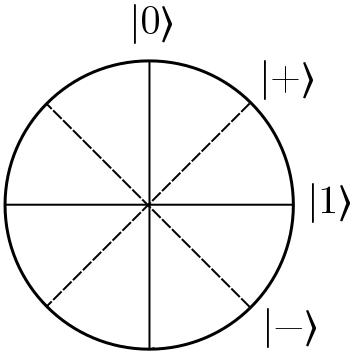
Polarisations of the photon, measuring in the horizontal/vertical ($01$) and diagonal ($+-$) bases.
Before we proceed, let’s quickly note a neat algebraic fact about the EPR pair. In the $+-$ basis, it looks pretty much the same as the $01$ basis, as a little algebra shows:
\[|\text{EPR}\rangle = \frac{1}{\sqrt{2}}(|0\rangle|1\rangle+|1\rangle|0\rangle)= \frac{1}{\sqrt{2}}(|+\rangle|-\rangle+|-\rangle|+\rangle).\]3.4. Sifting
Here is the new protocol. Alice and Bob can still pull EPR pairs from a common source, but now they randomly choose whether to measure normally (with outcomes $0$ and $1$) or rotate their devices (with outcomes $+$ and $-$). After measuring, they get on their intergalactic smartphones (or some other unsecure classical channel) and tell each other what basis they used, i.e. $01$ or $+-$. If they used the same basis, they will have opposite outcomes, from the properties of the EPR pair. In this case, they can figure out a shared bit and add it to their shared bit string.
If they choose different bases, they have to scrub the qubit, since neither can be sure what the other measured. For instance, if Alice uses the $01$ basis and measures $0$, the state becomes
\[|0\rangle|1\rangle = \frac{1}{\sqrt{2}}|0\rangle(|+\rangle - |-\rangle).\]If Bob measures in the $+-$ basis, he has a $50$-$50$ chance of observing either outcome, and Alice has no idea what he measures! By the same token, Bob can’t tell what Alice measured. The stage of the protocol — where they check basis and scrub some qubits — is called the sifting phase.
3.5. BB84
So far, this just seems like a more complicated version of the failed scheme from before. But unlike our earlier protocol, we now have the wherewithal to detect tampering. For argument’s sake, I’m going to assume that Alice and Bob flip a (classical) coin to determine which basis to measure their qubits in. To beat Eve, all they need to do is choose a subset of their shared bit string — remembering that for these bits to go into the shared string in the first place, Alice and Bob must have measured them in the same basis — and over the classical channel, reveal the actual measurement outcomes. If they happen to measure the same value, instead of the complementary values dictated by entanglement, Alice and Bob can tell that someone has been listening in.
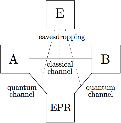
The setup for the BB84 protocol. Alice (A) and Bob (B) share a source (EPR) of EPR pairs; Eve (E) can eavesdrop on both classical and quantum transmissions.
Let’s see why. If Eve intercepts and measures a qubit (which Alice and Bob later measure in the same basis), she has to make a choice about which basis to measure in: $01$ or $+-$. She has a $50\%$ chance of making the same choice as Alice and Bob. If Eve makes the same choice as Alice and Bob later make, then as in the single basis protocol, her interference with that qubit goes undetected. Alice and Bob get complementary outcomes, and no alarm bells go off.
But suppose she makes a different choice, for instance, she chooses to measure in $01$ while Alice and Bob measure with $+-$. If Eve intercepts Alice’s qubit and measures a $0$, we get
\[|\text{EPR}\rangle \to |0\rangle|1\rangle = \frac{1}{2}(|+\rangle|+\rangle + |+\rangle|-\rangle - |-\rangle|+\rangle - |-\rangle|-\rangle).\]In other words, Eve’s measurement turns the state into a uniform probability distribution over all measurement outcomes in the $+-$ basis. That means there is a $50\%$ chance Alice and Bob choose different outcomes (no alarm bells), and a $50\%$ chance they choose the same outcome (alarm bells). Since Eve has a $50\%$ chance of choosing a different basis from Alice and Bob, and when she does, they still have a $50\%$ chance of getting opposite outcomes, Eve has a $1/4$ chance of being detected, and hence a $3/4$ chance of going scot free.
You may think they are pretty good odds for an eavesdropper. But all Alice and Bob need to do, to guarantee an arbitrarily high chance of detecting eavesdropping, is to sacrifice enough qubits from the shared string. For instance, if they sacrifice $15$ qubits, Eve has $1\%$ chance of going undetected. If they sacrifice $100$ qubits, Eve chances drop to $1$ in three trillion. That’s the BB84 protocol!
You can play around with a BB84 simulator online at QKD Simulator. If you do, you’ll see that there is much more to a practical QKD implementation than the bare bones outlines I’ve given. For instance, Alice and Bob can correct errors arising from noise in the EPR source, and importantly, distinguish these from an eavesdropper.
The reason I chose to talk about QKD today is that, although quantum computers use entanglement in a much deeper and more interesting way, key distribution is the most mature entanglement-based technology. EPR pairs are typically implemented as photon polarisations sent over optical fibres. The current state of the art is quite impressive. Recently, Chinese scientists broke the record for distance of entanglement transmission, sending halves of an EPR pair between ground stations over 1200 km apart via a satellite. Transmission rates get as high as $\sim 1$ Mbit/s. At that rate, Alice and Bob could encode a copy of War and Peace with a one-time pad, which is provably unbreakable, in under a minute. In the near future, I think we should expect to see satellite-based QKD become available to consumers. It’s an exciting time for quantum science!