May 3, 2016. A post on anyons (particles with fractional spin) and how they might be used in quantum computing. Based on a talk to undergraduates at the University of Melbourne.

Introduction

We’re told from kindergarten that particles come in two basic flavours: bosons and fermions. Bosons have integer spin and they’re social. When it gets cold, they like to clump together into giant, macroscopically degenerate atoms. Fermions, on the other hand, have half-integer spin and are the ultimate nonconformists, since the Pauli exclusion principle forces each one to have different properties from every other one! But there is more to life than bosons and fermions. In two dimensions, there is a whole new class of objects called anyons which are neither. I’ll show why anyons are allowed, give a simple physical model in terms of flux tubes, and finish by sketching how they can be used for quantum computing.

Bosons and fermions

Let’s remember how the division into bosons and fermions comes about. Suppose we have two identical particles at positions $P$ and $Q$. According to quantum mechanics, this system is described by a wavefunction $\Psi(P, Q)$, a complex-valued function of the two positions. We can write this in polar coordinates, separating out the amplitude and the phase:

\[\Psi(P, Q) = |\Psi(P,Q)|e^{i\theta(P, Q)}.\]

These are both physically meaningful:

• squaring the amplitude gives the probability of finding particles at $P$ and $Q$;
• the phase is responsible for interference effects, like water waves colliding in a pool or the double slit experiment.

Note that the phase itself is not physically meaningful, only differences in phase.

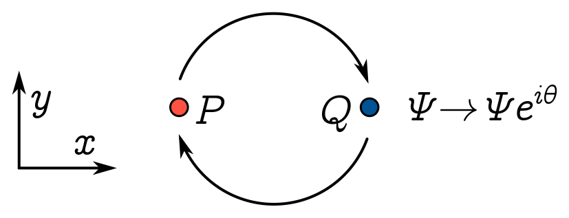
If you turn around, and I quickly swap the particles at $P$ and $Q$, could you tell that I’ve swapped them? The same types of particles are in the same spots, so any tests you perform on the system in isolation must give the same answer. In fact, precisely because the phase is unobservable, the only thing that can change is the phase; in isolation, we can’t detect it. Let’s suppose that when I swap the particles, the wave function picks up a phase factor $\Psi \to \exp(i\theta)\Psi$. To figure out the phase, you would need to do quantum interference experiments with copies of the system before and after swapping.

But we can perform a thought experiment which is almost as good, and dramatically narrows down the options for $\theta$. (We still need to do an experiment to see which option any given system takes though.) Suppose we swap twice, producing a phase factor $e^{2i\theta}$:

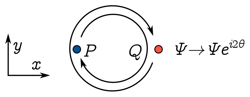
But swapping twice gives the original system back, with the same particles in the same place, not just the same type of particle in the same place. The wave function should threfore be exactly the same, phase and all, so $\Psi e^{2i\theta} = \Psi$.

Since $e^{2i\theta} = 1$, we must have $e^{i\theta} = \pm 1$. Bosons are particles whose wavefunctions don’t change when we swap particles, so $e^{i\theta} = +1$. That means the phase $\theta = 2n\pi$ for some integer $n \in \mathbb{Z}$. Fermions are particles which pick up a minus sign under swapping $e^{i\theta} = -1$, so the phase $\theta = (n+1/2)2\pi$ for some half-integer $n+ 1/2$. The integer or half-integer sitting in the phase is called the spin of the particle, so we learn that bosons have integer spin and fermions half-integer spin.

Two further points. First of all, you may object that, based on what we’ve said so far, I have no way of distinguishing bosons of different spin. It’s beyond the scope of this talk, but one way to figure this out is to see how a particle behaves when you change to a different reference frame. Secondly, you might wonder if the $2\pi$ in the phase has a geometric meaning, and indeed it does. In doing the swap, we rotated each particle by $\pi$ around the common centre, so the “total” angle is $2\pi$. A more general statement, then, is that each particle picks up a phase of $s\Phi$, where $\Phi$ is the angle we rotate it through and $s$ is the spin. You now know a baby version of the spin-statistics theorem!

Anyons

I said before that swapping a pair of particles twice gives you back the original system. But do you buy that? Couldn’t swapping twice lead to a nonvanishing phase? When I do the double swap, I can think of physically moving the particles along paths which implement the swapping. Perhaps I continuously measure the particles to localise to those paths, and have some nonzero chance of success. But I shouldn’t really care about the exact choice of path, since I can’t exactly localise them anyway. It follows that any phase changes should be the same if I continuously deform the path. But that means I can continuosly pull one loop over the other, and then shrink both: no more loops!

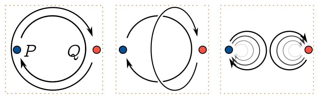
This means that swapping twice really is equal to doing nothing, if you buy the argument that deforming loops doesn’t change the phase. But there is a loophole (pun intended) in the argument I’ve just given. I’ve assumed something about space, namely that we can move the loops around in three dimensions. But in flatland, I can’t contract the big loop, since I’m not allowed to lift anything out of the page. Aall my fine arguments about double swaps go out the window, and there are no longer any restrictions on the phase factor under a swap. We learn that in 2D, $\Psi \to e^{i2 \pi a}\Psi$ is allowed for any real number $a$.

This zoo of particles with unconstrained spin are called anyons, since they can have any spin. Let’s see how these arise in reality.

Aharanov-Bohm effect

Our first example is the Aharanov-Bohm effect. The basic setup is that we have some charge $q$ moving around in a plane, and a tube of magnetic flux which intersects that plane:

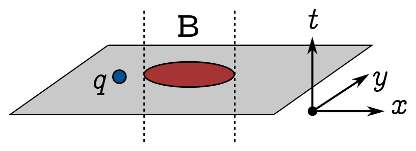
Since there are no magnetic charges (or at least, we haven’t seen any), $\nabla\cdot\mathbf{B} = 0$ and vector calculus guarantees we can write the magnetic field as the curl of some vector field $\mathbf{A}$, which we call the vector potential:

\[\mathbf{B} = \nabla \times \mathbf{A}.\]

Let’s switch the magnetic field off by setting $ \mathbf{A} = \mathbf{0}$. If there are no other forces, the charged particle can freely propagate and has wavefunction $\Psi_0(\mathbf{r})$.

\[i \frac{\partial \Psi}{\partial t} = \hat{H}\Psi = \frac{\hat{p}^2}{2m}\Psi = -\frac{\hbar^2}{2m}\nabla^2\Psi.\]

Now switch the magnetic field back on. Interestingly, all that happens to the old wavefunctions is that they pick up a phase factor:

\[\Psi(\mathbf{r}) = \exp\left[\frac{iq}{c\hbar} \int_{\mathbf{r}_0}^{\mathbf{r}} \mathbf{A} \cdot d\mathbf{r}\right]\Psi(\mathbf{r}),\]

where we integrate from an arbitrary reference point $\mathbf{r}_0$. In other words, by simply plonking a line integral into the phase, we can recycle our solutions to the free Schrödinger equation to get the wavefunction for a charged particle in a magnetic field. But this should be ringing some bells—we have a phase factor which depends on a path, just like spin-statistics. Pursuing this connection, let’s run the charged particle in a loop $\ell$ around the flux tube:

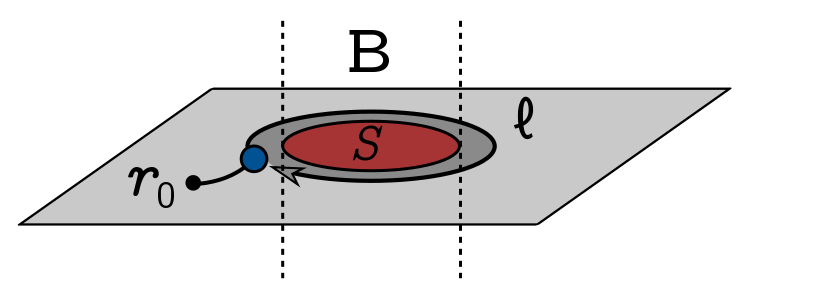
The wavefunction picks up an additional phase

\[\begin{align*} \exp\left[\frac{iq}{c\hbar} \oint_\ell \mathbf{A} \cdot d\mathbf{r}\right] & = \exp\left[\frac{iq}{c\hbar} \int_S (\nabla\times \mathbf{A}) \cdot d\mathbf{S}\right]\\ & = \exp\left[\frac{iq}{c\hbar} \int_S \mathbf{B} \cdot d\mathbf{S}\right] \\ & = \exp\left[ \frac{iq}{c\hbar}\Phi_B\right] \end{align*}\]

where we’ve used Stokes’ theorem to convert the line integral around the loop $\ell$ to a surface integral over $S$, the region it encloses. Here, $\Phi_B$ denotes the magnetic flux through the loop, so the phase factor is just a multiple of the enclosed flux. If the flux is localised to a small patch of the surface (as in the picture), you can deform the loop without affecting the phase acquired.

If we combine the two active ingredients here — the flux tube and the charge — into a single object, we effectively get an anyon. It can cause phase changes due to the flux, and it can undergo phase changes because it’s charged. So this is one simple way to implement them in 2D! Turning things round, we can argue as above that in three (and higher) spatial dimensions, flux is quantised. It comes in units of the flux quantum $\Phi_0 = \hbar c/q$.

Braids and fusion

Now we’re going to move on to the fun part of the talk, where we see how to combine anyons together and do computations with them. We can visualise how a system of anyons evolves in time using braids. Take a bit of paper, and glue $n$ strands of string to the bottom in a line. Now imagine knotting them together by twisting adjacent threads together as many times as you like. Glue the $n$ dangling strands to another piece of paper.

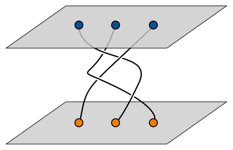
The resulting structure is called a braid. The specific positions of the strings is unimportant: all that matters is the topology or order of the twists. What has this got to do with anyons? The top piece of paper describes the initial positions of $n$ anyons, and the bottom piece of paper the final positions. All the braiding in between tells you how the anyons moved around each other between the initial and final time. They’re paths for the anyons to move along.

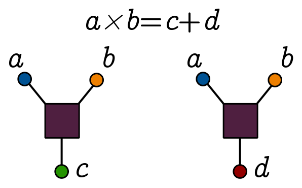
Another key operation on anyons is fusion. This just means putting two anyons $a$ and $b$ into a box and seeing how the combination behaves. For instance, it could behave like some other anyon in our system, $c$. It might be that there are different outcomes for fusion: putting $a$ and $b$ in a box sometimes behaves like $c$ and sometimes like $d$. We denote fusion by $\times$, and different fusion outcomes by $+$, so that $a \times b = c + d$. We represent anyons by labelled legs, and fusion as a box with inputs, as below:

When we braid anyons, the system picks up different phase factors which can be assigned to a big matrix called the $R$ matrix. When we fuse in different ways, we can relate the outcomes using another big matrix called the $F$ matrix. (If you like, $R$ encodes the penalty for commuting anyons, and $F$ tells you precisely how associativity of fusion fails.) The $R$ and $F$ matrices encode all the information about a system of anyons. They obey some nice relations which follow from the equivalence of certain sequences of braiding and fusion, naturally expressed in the language of category theory. Unfortunately, that is beyond our current scope.

Topological quantum computers

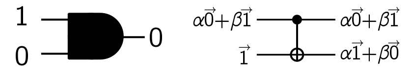
We now know enough about anyons to build a (hypothetical) quantum computer with them. One way to think about quantum computers is as a generalisation of logic circuits. In a logic circuit, you compute with binary digits (bits) $0$ and $1$. These could correspond to current flowing or no current flowing in a wire. Using logic gates like AND, OR, and NOT, you can harness the bits flowing around the circuit to calculate stuff. In a quantum computer, bits are replaced by quantum bits (qubits), which are quantum superpositions of $0$ and $1$. Logic gates are replaced by quantum gates, which are basically matrices acting on the vector representing a qubit. For instance, below we compare the classical AND gate, acting on regular bits, to the CNOT gate, which acts on linear combinations of bits as shown:

To physically implement a quantum circuit, we need to do three things. First of all, we need to create the input state for the problem we want our circuit to solve. (For instance, you might want factorise a particular large number.) Next, we need to physically implement the quantum gates that make up our circuit. Finally, we need to read the result of our computation out of the system, that is, make a measurement of the final state and extract information from it. Of course, this is a dramatic simplification of what’s involved, but you get the idea!

In a topological quantum computer, we can do each of these things with anyons. To create input states, we need a scheme for encoding qubits as anyons, and a physical mechanism for producing specific anyon states. Quantum gates are achieved by a judicious combination of braiding and fusion. At the end of the computation, you fuse all the anyons in the system, and use our knowledge of the $F$ matrix to see what was probably in the final state. If you run the circuit multiple times, you can figure out the answer with arbitrarily high probability (as long as everything works as I’ve described).

Of course, in reality quantum computers are extremely vulnerable to noise. Interactions with the environment, or unintended interactions between parts of the system, can lead to a loss of quantum state, or even the destruction of the anyons themselves. The nice thing about braiding and fusion is that both are somewhat resilient to local errors. I can deform a path or wiggle a box of anyons without changing the computational outcomes. This property is called topological stability, and it’s one of the key reasons anyons are interesting to people in the quantum computing community.

Fibonacci anyons

I’ll finish with a very cute computational scheme using Fibonacci anyons. Here, we just have a single anyon type $\tau$, and the vacuum state, denoted $1$. There are two fusion rules:

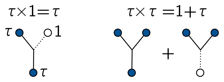
The first rule says that an anyon in a box by itself is still just an anyon. But if you put two anyons in a box together, they can either annihilate (giving $1$) or fuse to form a single anyon $\tau$. Using constraints on the $R$ matrix, you can actually work out that the $\tau$ anyon has spin 11/10!

Let’s talk about how to compute things. You can fuse three $\tau$ anyons to form a single anyon (label this $3\tau \to \tau$) in two different ways:

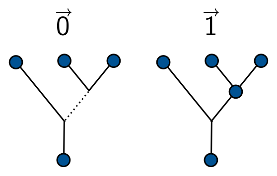
Basically, we fuse two anyons, and either get an anyon or nothing; we then fuse the result with another anyon, and throw away the result if we don’t end up fusing. So we have two options, depending on the result of our first fusion. These two options encode the two bits, $0$ and $1$, and we can take quantum superpositions to get an arbitrary qubit. Incidentally, you can continue counting ways to achieve $(n - 1)\tau \to \tau$. This turns out to be the $n$th Fibonacci number! I’ll leave it as an exercise for reader, but I mainly wanted to explain where the name comes from. (Hint: If you consider the number of ways to fuse $n - 2$ anyons to get a $\tau$ anyon or a vacuum state, you should end up with the Fibonacci recursion.)

Our quantum gates are implemented are built out of two basic operations: a simple swap of two $\tau$ anyons, and the more elaborate act of creating two pairs of anyons from the vacuum, braiding one from each pair, then fusing both pairs to end up with two anyons:

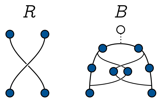
The first is described by the $R$ matrix, the second by a combination of the $F$ and $R$ matrices I just call $B$. It turns out you can approximate any quantum gate you like using products of $B$ and $R$ matrices. Finally, when you fuse all the anyons at the end of the computation, you want to run the encoding scheme in reverse and figure out what qubits were floating around in the final state.

Obviously I’ve swept a lot of details under the rug. But to reiterate the main points: in flatland, particles can have any spin; one way to implement anyons physically is to combine a charged particle with a flux tube; and finally, we can fuse and braid anyons to make a topologically robust quantum circuit.

References

• Topological Quantum Computing (2015). Janos Pachos.
• Quantum Computation and Quantum Information (2010). Michael Nielsen and Isaac Chuang.
• “A short introduction to Fibonacci anyon models” (2009). Simon Trebst, Matthias Troyer, Zhenghan Wang, Andreas W.W. Ludwig.