Hacking physics from the back of a napkin
February 24, 2020. The computational power of a humble napkin is awesome. I discuss three napkin algorithms — dimensional analysis, Fermi estimates, and random walks — and use them to figure out why rain falls, the length of the E. coli genome, and the mass of a proton, among other things. These examples suggest a napkin-based approach to teaching physics.
Contents
1. Hacking physics
Hacker spirit. Nowadays, the word “hacker” conjures up visions of Russian trolls, Julian Assange, and Angelina Jolie’s 90s pixie cut. But a nobler usage predates this. Hacker culture, in the original sense, grew out of places like MIT in the 60s, with its tradition of highbrow silliness and elaborate technical pranks. Although associated with programming, hacker spirit can be viewed as a broader ethos about play, understanding and creativity. In the words of open-source gnuru Richard Stallman,
What [hackers] had in common was a love of excellence and programming. They wanted to make the programs that they used be as good as they could. They also wanted to make them do neat things. They wanted to be able to do something in a more exciting way than anyone believed possible and show ‘Look how wonderful this is. I bet you didn’t believe this could be done.’
Using techniques in a clever or unexpected way is a hack, with hack value quantifying the degree of ingenuity. (“Hack” is actually a back-formation of “hack value”.) Hackers do not look for the most powerful, or obvious, or easy tool for the job. They delight in the unexpected, in using humble means to achieve extraordinary ends. In a way, they realise David Deutsch’s definition of knowledge as information with causal power. Knowing a technique well enough to hack it means you can act on the world in new ways.
I think physics needs more hacker spirit: more people willing to fool around and explore what our marvellous toolset can do, to creatively defy expectations and push the Deutschian envelope. Physics is not withouts its hackers but unlike computer science, the hackers are colourful exceptions, tending towards goofy irreverence and self-mythology (Richard Feynman springs to mind). I think hacking should go mainstream.
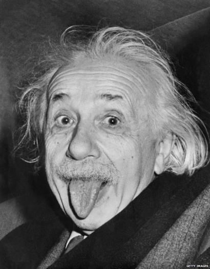
Napkin hacks. My goal in this post is to outline a few simple hacks for the back of a napkin. I think of these as algorithms for a napkin computer, and with some practice, they really can be implemented using high school algebra on a small piece of paper, without calculus or calculators (though the latter save time). While there is whimsy and irreverence aplenty, our focus will be real physics. Our goal will be a beautiful proof of the existence of atoms, due to none other than Albert Einstein, the greatest physics hacker of all. Another running theme is rain, a tribute to my rainy city of residence, Vancouver.
Hackery is not just about excellence and creativity for their own sake, but has clear pedagogical implications. Most people have to wait until grad school to compute viscous drag, estimate urban power usage, or determine the size of the E. coli genome. But imagine a world where high school students are so empowered that, given a few hints, a pencil, and a napkin, they could discover it all themselves. This world is very close to ours: all we need is a little more hacker spirit in the enjoyment and instruction of physics.
Notes. This post really consists of three distinct tutorials. The dimensional analysis tutorial and section on Fermi estimates can be read independently. The last tutorial on random walks assumes you have read the dimensional analysis section. The exercises are just as important as the text, but only the results of Exercise 3 and Exercise 14 are used subsequently. Solutions, and various other technicalities, are collected here.
2. Dimensional analysis
We will start with one of the most powerful but underappreciated tools in physics: dimensional analysis. Physics is ultimately about experimental measurements. Take some object, maybe an old pumpkin, and poke or prod it with a measuring device. The device returns a number, but that’s not what interests us; instead, we want to know the physical property probed by that device. This is what we mean by dimension. For instance, if we compare the width of the pumpkin to a ruler, the dimension is the length, if we put it on some scales it’s the mass, and if we time how long it takes to rot, the dimension is time.
We denote the dimension of length by $L$, time by $T$ and mass by $M$. We use brackets $[\cdot]$ to refer to the dimension of a measurement. It’s easy when the measurement is given in some units, since we can throw away the numbers and just ask: what aspect does the unit measure? For instance,
\[[20 \text{ cm}] = [\text{cm}] = L, \quad [5 \text{ lb}] =[\text{lb}] = M, \quad \quad [2 \text{ days}] =[\text{days}] = T.\]Centimetres measure length, hours measure time, and pounds measure mass. More complicated dimensions follow from the basic ones according to simple rules which are easier to show than tell. Area, for example, has dimensions $L^2$:
\[[1 \text{ cm}^2] = [\text{cm}^2] = [\text{cm}]^2.\]An alternative to units is using general formulas, e.g. for the area of a rectangle:
\[[\text{area}] = [\text{width}\times \text{height}] = [\text{width}] \times [\text{height}] = L^2.\]Dimensions can be divided as well as multiplied:
\[[\text{velocity}] = \left[\frac{\text{distance}}{\text{time}}\right] = \frac{[\text{distance}]}{[\text{time}]} = \frac{L}{T}.\]Be careful: only measurements with the same dimensions can be added and subtracted. For instance, it makes no sense to ask what “$1$ cm + $4$ hours” is, though it is sensible to compute “$1$ cm + $4$ feet”.
Physical laws tell us how measurements depend on each other. For example, Newton’s second law $F = ma$ tells us how measurements of force, mass and acceleration are related. If the two sides of $F = ma$ are equal, the dimensions must agree, with
\[[F] = [m a] = [m]\times \left[\frac{v}{t}\right] = \frac{ML}{T^2}.\]The point of dimensional analysis is that you can sometimes reverse this process, and determine the physical laws from dimensions! Let’s see how.
2.1. Pendulous pumpkins
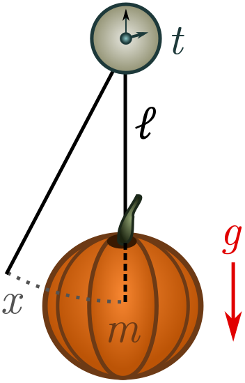
Suppose we attach an old pumpkin to a length of string and give it a kick. Gravity will pull on the pumpkin, causing it to oscillate back and forth with some period of oscillation $t$. If we know how the period of oscillation depends on other properties of the system, we can utilise this knowledge to make a pumpkin clock! Let’s start by listing some relevant quantities:
- the mass of the pumpkin $m$, with dimension $[m] = M$;
- the length of the string $\ell$, dimension $[\ell] = L$;
- gravitational acceleration $g = 9.8 \text{ m/s}^2$, dimension $[g] = LT^{-2}$ (from the units);
- the initial displacement of the pumpkin $x$, dimension $[x] = L$.
Not all of these quantities will turn out to be relevant. Galileo discovered that as long as the initial kick is small, it has no affect on the period: pendulums are “isochronic”. Grab a pumpkin, stopwatch and string, and check for yourself! Galileo realised he could exploit this property to make a reliable timepiece, and invented the pendulum clock. (There is actually a deep physical reason pendulums are isochronic for small kicks, but we will have to leave that for another time!)
In terms of relevant features, this leaves the pumpkin mass $m$, string length $\ell$, and gravity $g$. You can also eliminate the pumpkin mass empirically, but as we’ll see, we can leave it in and let dimensional analysis tell us it’s irrelevant. At this point, I’m going to do something a bit sneaky. Instead of period $t$, we will deal with the angular velocity
\[\omega = \frac{2\pi}{t}.\](We will explain another way to get factors of $2\pi$ in Exercise 4.) Dimensional analysis is nothing fancier than guessing that $\omega$ is related to $m$, $\ell$ and $g$ by an equation of the form
\[\omega = m^a \ell^b g^c,\]for some numbers $a$, $b$, and $c$. Our goal is to figure out what these numbers are. We can find the powers by matching dimensions on each side:
\[\begin{align*} \frac{1}{T} = [\omega] = [m^a \ell^c g^c] = \frac{M^aL^{b+c}}{T^{2c}}. \end{align*}\]Requiring the leftmost and rightmost expressions to be equal, we can immediately read off the powers:
\[a = 0, \quad 2c = 1, \quad b + c = 0 \quad \Longrightarrow \quad a = 0, \quad c = -b = \frac{1}{2}.\]As promised, dimensional analysis kindly informs us that the mass is irrelevant! My earlier piece of sneakiness (replacing period with angular velocity) actually gives the exact answer for small kicks:
\[\omega = m^a \ell^b g^c = \sqrt{\frac{g}{\ell}}.\]We didn’t need to solve a differential equation, analyse forces, or even deal with numbers. Dimensional analysis let us skip straight to the answer!
Suppose we want to make a pumpkin clock with the conventional grandfather-clock period of $t = 2 \text{ s}$, so that each half swing takes one second. Then we should suspend the old pumpkin from a string of length
\[\ell = \frac{g}{\omega^2} = \frac{g t^2}{(2\pi)^2} = \frac{9.8 \text{ m}}{\pi^2} \approx 1 \text{ m}.\]Incidentally, this explains why grandfather clocks are so large. They will house a large (typically non-curcurbitar) pendulum with $\ell \approx 1$ m.
In order to make the clock, we need a ruler to measure out the length of string. But for maximal whimsy, we can switch things up, and turn a stopwatch, pumpkin and spool into a ruler! Measure with the string and snip off the corresponding length, attach the pumpkin and gently wobble. By timing the period with the stopwatch, you can figure out how long things are. Exercise 1 is another whimsical pumpkin-as-ruler example, involving Kepler’s third law!
Exercise 1 (interplanetary pumpkins). You can use an old pumpkin to measure very large objects. Place the sun at one end and the pumpkin at the other. If you kick the pumpkin with enough energy tangent to the sun, it will orbit in a circle of radius $r$ (the length of the object) with angular velocity $\omega$. You may have to kick many times until this happens!
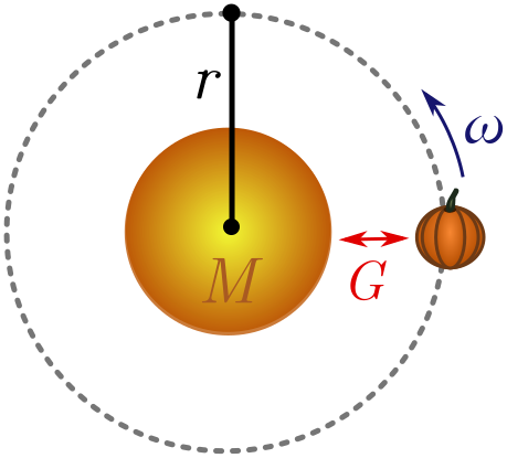
Using dimensional analysis, show that
\[r \sim \left[\frac{GM_\odot}{\omega^2}\right]^{1/3},\]where $M_\odot$ is the mass of the sun and $G = 6.7 \times 10^{-11} \text{ m}^3 \text{/kg s}^2$ is Newton’s constant, controlling the strength of gravity. This relation is Kepler’s third law!
Hint. You can ignore the mass of the pumpkin due to the equivalence principle: objects fall the same way in gravitational fields, whatever their mass.
2.2. Drag and drop
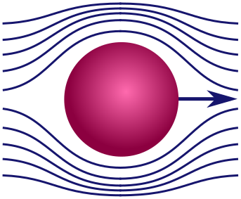
Stokes’ law. Maybe pumpkins aren’t your thing, so let’s turn to something more highbrow: the aerodynamics of spheres. Realistic fluids have a sort of internal stickiness called viscosity, responsible for making honey so goopy and delicious. Because of viscosity, a fluid will resist our efforts to pull layers of fluid in different directions, or shear them. This is similar to the way friction resists the motion of one surface against another.
A sphere moving through fluid splits the layers at the front, then joins them at the back, a bit like a zipper. This is a shearing force and will lead to viscous resistance. Our goal will be to determine the precise drag force on the sphere. Here are some factors that might be relevant:
- the radius of the sphere $r$, with $[r] = L$;
- the speed of the sphere $v$, where $[v] = LT^{-1}$;
- the mass of the sphere $m$, $[m] = M$;
- the density of the fluid $\rho$, or mass per unit volume $[\rho] = [m_\text{fluid}/V] = ML^{-3}$;
- the viscosity of the fluid $\mu$.
In general, all of these factors are involved, but this is too much for dimensional analysis to handle! (I’ll explain why below.) So what can we do?
Thankfully, if the sphere moves very quickly or very slowly, certain factors dominate, and the list becomes short enough to use dimensional analysis. When the sphere moves very quickly, it is banging water molecules out of the way rather than smoothly shearing. In this case, the mass of the sphere $m$ and the density of fluid $\rho$ are important, but viscosity is not. (You can explore this scenario in Exercise 2.) We will look at the opposite regime, where the sphere moves very slowly. In this case, the sphere smoothly shears through the water without collisions, so neither $m$ nor $\rho$ are relevant. Drag is dominated by the viscosity $\mu$ and the geometry of the sphere. This force would be present, even if both where arbitrarily light!
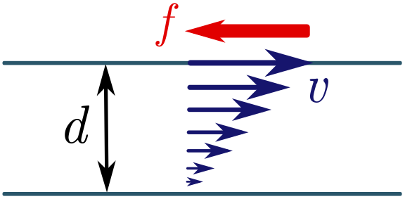
I haven’t told you the dimensions of viscosity yet, but we can find them fairly easily — assuming we have a fluid mechanics lab! I’ll save you the trouble of doing the experiments and tell you what happens. Suppose we have two layers of fluid flow separated by a distance $d$, and I try to shear them by moving one layer parallel to the second at speed $v$. Experiment shows that the fluid will resist with some force $P = F/A$ per unit area, proportional to $v$ and inversely proportional to the separation $d$. The viscosity $\mu$ is the constant of the proportionality, so
\[P = \frac{F}{A} = \mu \left(\frac{v}{d}\right) \quad \Longrightarrow \quad [\mu] = \left[\frac{dF}{Av}\right] = \frac{L(ML/T^2)}{L^2(L/T)} = \frac{M}{LT}.\]If you skipped the previous paragraph, that’s fine, as long as you are prepared to take the dimensions on faith. Either way, we can proceed with our dimensional analysis. Let’s write the drag force on the sphere $F_\text{drag}$ as a product of powers of the remaining factors:
\[F_\text{drag} = r^a v^b \mu^c.\]Then
\[\frac{ML}{T^2} = [F_\text{drag}] = [r^a v^b \mu^c] = L^a \cdot \left(\frac{L}{T}\right)^b \cdot \left(\frac{M}{LT}\right)^c = \frac{L^{a+b-c}M^c}{T^{b+c}}.\]On the LHS, mass appears as $M^1$, so $c = 1$. The LHS has time appearing as $1/T^2$, so
\[b+c = b+1 = 2 \quad \Longrightarrow \quad b = 1.\]Finally, the LHS has length appearing $L^1$, and comparing to the RHS gives
\[a + b -c = a = 1.\]Dimensional analysis tells us that the drag force is
\[F_\text{drag} \sim \mu^a r^b v^c = \mu r v.\]As usual, we can’t determine if there is a number out front. With considerably more work, George Stokes showed that
\[F_\text{drag}= 6\pi \mu r v.\]This is called Stokes’ law in honour of its discoverer. But we got pretty darn close with a few lines of algebra!
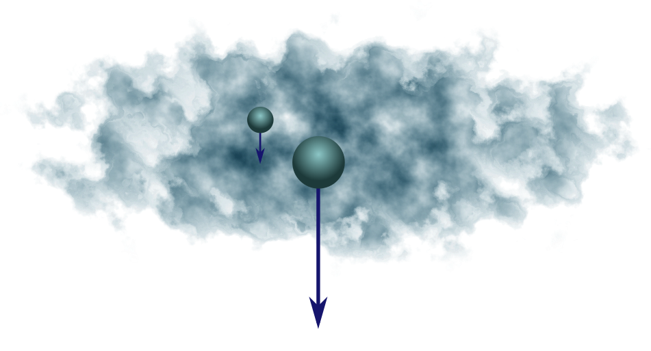
Why clouds float. We finish this example by calculating the terminal velocity of water droplets in a cloud. This will help explain why clouds float and rain falls! First, consider the general case of a slowly falling sphere. A sphere of mass $m$ is pulled down by the weight force $F_\text{weight}= mg$. If it’s moving slowly, Stokes’ law applies and the drag force is proportional to the velocity, $F_\text{drag} = 6\pi \mu r v$. The terminal velocity $v_{\text{term}}$ is the speed at which these two forces balance out:
\[F_\text{weight} = mg = 6\pi \mu r v_{\text{term}} = F_\text{drag}\quad \Longrightarrow \quad v_{\text{term}} = \frac{mg}{6\pi \mu r}.\]The sphere accelerates until it reaches $v_{\text{term}}$. Since we’re going to be interested in spheres of water of different sizes, let’s trade in mass for the density $\rho$:
\[m = V\rho = \frac{4\pi r^3}{3} \rho \quad \Longrightarrow \quad v_{\text{term}} = \frac{mg}{6\pi \mu r} = \frac{2\rho r^2 g}{9\mu}.\](You can also take buoyancy forces $F_\text{buoy} = V \rho_\text{fluid}$ into account, where $\rho_{\text{fluid}}$ is the density of the fluid. This just replaces $\rho$ with $\rho - \rho_{\text{fluid}}$. Since water is much denser than air, the buoyancy forces in our case are negligible.)
The density of water is $\rho \approx 10^3 \text{ kg/m}^3$, and a typical droplet of water vapour has a radius around $r = 2\times 10^{-5} \text{ m}$. Finally, the viscosity of air is $\mu \approx 2\times 10^{-5} \text{ kg/m s}$. The terminal speed of a cloud droplet is therefore
\[v_{\text{term}} = \frac{2\rho r^2 g}{9\mu} = \frac{2(2\times 10^{-5} \text{ m})^2(10^3 \text{ kg/m}^3)(9.8 \text{ m/s}^2)}{9(2\times 10^{-5} \text{ kg/m s})} \approx 0.04 \text{ m/s},\]or $4$ centimetres per second. It requires only mild updrafts of warm air (rising from the warmer regions near the ground) to keep the cloud aloft. Stokes’ law also explains why rain falls. The terminal velocity $v_\text{term} \propto r^2$, increasing quickly as droplets get larger. If droplets coalesce (for example, with water vapour arriving in an updraft) they will speed up and fall out of the cloud. Voilà, rain!
Exercise 2 (terminal raindrops). When a raindrop gets big enough to fall out of a cloud, it is no longer moving slowly, and Stokes’ law does not apply.
(a) Raindrops fall fast enough that the viscosity of air is irrelevant, but the density $\rho_\text{air}$ is. Repeat the analysis above to find that the drag force on a raindrop of size $r$ is
\[F_\text{drag} \sim \rho_\text{air} v^2 r^2.\](b) Conclude that the terminal velocity for a spherical raindrop of radius $r$ is
\[v_\text{term} \sim \sqrt{\frac{4\pi g r}{3 }\left(\frac{\rho_\text{water}}{\rho_\text{air}}\right)}.\](c) A typical raindrop has radius around $r \approx 1$ mm. How fast does it hit the ground?
2.3. Usage notes
Numbers. Dimensional analysis has its limits. First of all, it can be wrong by an overall numerical factor. In Stokes’ law, for instance, we were off by $6\pi \approx 20$, and if we used period rather than angular velocity, our earlier examples would be off by $2\pi \approx 6$. That said, more often than not the missing number is close to $1$, and we can even dimensionally account for some factors of $\pi$ (Exercise 4).
Parametric overload. A more serious problem is having too many parameters. With three basic dimensions $M, L, T$, you can have at most three relevant parameters, since each parameter comes with an unknown $(a, b,c)$ and each dimension gives us an equation. Three equations is just right for three unknowns. Any more unknowns, and you don’t have enough equations to determine them all! There are further subtleties, but they are all captured in a nice result called the Buckingham $\pi$ theorem. For a very elementary treatment, see my detailed notes on dimensional analysis.
Where is the physics? You might think that dimensional analysis is algebra rather than physics. But to avoid parametric overload, we need to whittle down our factors until we have a manageable number. Sometimes we can do this by physical reasoning (e.g. the equivalence principle in Exercise 1), or restricting to situations where factors are negligible (e.g. a slowly moving sphere). Sometimes, neither of these works, and we just have to go out, do experiments, and see how things vary (e.g. isochronism and viscosity). None of these operations necessarily involves hard maths, but they are definitely all physics!
Extra dimensions. Length, mass and time are not the only basic dimensions. Two other important dimensions are temperature $\Theta$ (measured in Celsius or Kelvin for instance) and amount of stuff $N$ (usually measured in mol). These are crucial in atomic physics, thermodynamics and chemistry. We will introduce them properly in Exercise 3, and lean heavily on them for the tutorial on random walks.
Constants. Numbers are dimensionless constants. However, dimensionful constants secretly encode physics! Examples include Newton’s constant $G$ (Exercise 1) and Boltzmann’s constant $k_B$ (Exercise 3). See my notes for applications of fundamental constants to black holes!
Exercise 3 (ideal gas law). A gas of $\mathcal{N}$ particles takes up space (with volume $V$), presses on its container (with pressure $P$), and is hot (with temperature $\mathcal{T}$). These properties are not independent! Their relationship is revealed by dimensional analysis.
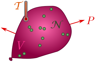
(a) Explain why volume should have dimension $[V] = L^3N$.
(b) Show that pressure has dimension $[P] = M/LT^2$.
(c) In thermodynamics, there is a fundamental constant called Boltzmann’s constant, $k_B = 1.38 \times 10^{-23} \text{ J/K}$, where $\text{K}$ stands for Kelvin. Confirm that $k_B$ has dimension
\[[k_B] = \frac{ML^2}{T^2\Theta}.\](d) Finally, use dimensional analysis to deduce the ideal gas law:
\[PV \sim \mathcal{N}k_B\mathcal{T}.\]In fact, the two sides are actually equal for a dilute gas! We will use the equals sign for the rest of the post.
⁂
Exercise 4 (factors of $\pi$). We can sometimes account for factors of $\pi$ by giving a dimension to angles. Suppose we have a system repeating itself in time periodically, e.g. a swinging pendulum or a planetoid orbiting the sun. We can keep track of where the system is in its cycle using an arrow moving around a unit circle at constant speed, with one revolution per cycle of the system. The arrow (called a phasor if you want to be fancy) subtends an angle of $360^\circ$ over the course of a single period, so really, a period should be viewed not as a time, but a time per $360^\circ$.
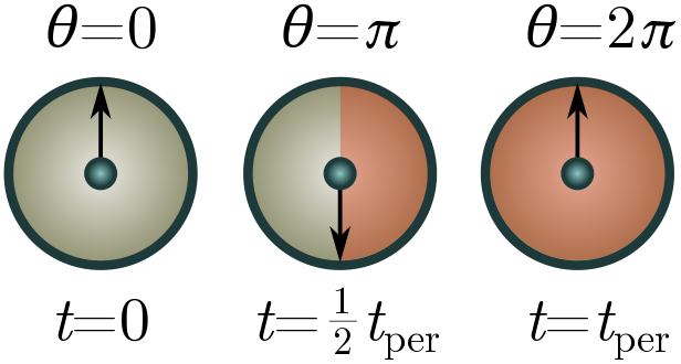
Let $[1^\circ] = \Xi$ be the dimension of angle, so that a period has dimension $[t_\text{per}] = T/\Xi$. This will leave factors of $\Xi$ floating around. To cancel them, we can view $2\pi$ as a “fundamental physical constant” with dimension $\Xi$. This isn’t totally crazy, since $360^\circ = 2\pi$ radian!
(a) Repeat the pumpkin problems above, now using $[t_\text{per}] = T/\Xi$ and $2\pi$ as a conversion factor. You should obtain the same results!
(b) If your system executes $n$ cycles in the process you’re considering, what conversion factor should you use instead of $2\pi$?
(c) The $6\pi$ in Stokes’ law does not come from a period. Where could it come from?
3. Fermi estimates
Our next napkin algorithm, Fermi estimation, is particularly strong with hacker spirit. A Fermi estimate is a guess accurate to the nearest order of magnitude, i.e. rounded to the nearest power of $10$. So, viewed through this generous lens, there are $10$ planets, $100$ countries, and $10$ billion people on the planet. The finer points of planetary science, geopolitics, and global census do not affect these guesses!
The nearest power of $10$ is actually a subtle concept. For instance, is $4$ closer to $1$ or $10$? If we use a normal or linear ruler, the answer is clearly $1$. But when we are rounding to the nearest power of ten, we do not have ticks at $0$, $1$, $2$, and so on, but at powers:
\[10^0 = 1, \quad 10^1 = 10, \quad 10^2 = 100, \ldots\]We should therefore use a logarithmic ruler, where we take logs in base $10$ and round to the nearest tick, where a tick now represents a power. In our case, $\log_{10}4 \approx 0.6$ is closer to $1$ than to $0$, and so $4$ rounds up to $10^1 = 10$! This is a bit surprising, but just the way things work when you think in Fermi … termies.
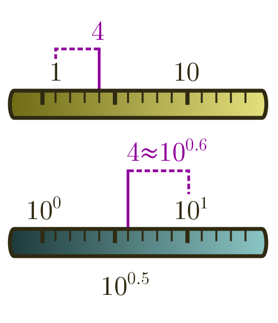
Anyway, on a linear ruler, if there is a tick for every whole number, rounding to the nearest tick means there is a possible error of $0.5$. In the same way, rounding to the nearest tick on a logarithmic ruler has an error of half a tick. But this really means half a power of $10$:
\[10^{0.5} \approx 3.2.\]An accurate Fermi estimate can be bigger or smaller than the true answer by a factor of $3$. Our earlier counts of planets, countries, and global population, for instance, are well within this generous margin of error!
In general, it makes life a bit easier if instead of restricting to power of $10$, we allow for arbitrary numbers, with the understanding that they are only accurate up to a factor of $10^{0.5} \approx 3.2$. We can denote this using a twiddle, so that
\[\text{number of countries} \sim 200\]means “we guess the number of countries is $200$, possibly up to a factor of $3$”. (When we do dimensional analysis, we also use a twiddle. In both cases, we are saying “up to some numbers out the front that are hopefully small”.) Now you know what a Fermi estimate is, let’s learn how to do them!
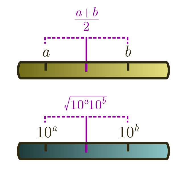
3.1. Geometric means
On a linear ruler, we average two numbers $a$ and $b$ by halving the sum, $(a+b)/2$. On a logarithmic ruler, we take logs first, then average. But what does this correspond to when we undo the logs? Let’s check, using log laws. First, from $\log x + \log y = \log xy$ and $n \log x = \log (x^n)$, we have
\[\frac{1}{2}(\log_{10} a + \log_{10} b) = \frac{1}{2}\log_{10} ab = \log_{10}\sqrt{ab}.\]From the log law $10^{\log_{10} x} = x$, it follows that
\[10^{(\log_{10} a + \log_{10} b)/2} = 10^{\log_{10} \sqrt{ab}} = \sqrt{ab}.\]This is called the geometric mean. Whenever you are dealing with estimates spread across different orders of magnitude, this is better to use than the usual arithmetic mean $(a+b)/2$. The arithmetic mean will just return the bigger number!
Geometric means are useful for averaging an underestimate and an overestimate. For instance, if we wanted to guess how many people have been to the moon, $1$ is clearly an underestimate, and $100$ seems like an overestimate. The geometric mean is
\[\text{moon people} \sim \sqrt{1 \cdot 100} \approx 10.\]The answer is actually $12$, so our guess is more or less on the mooney!
Calculation tips. You might be wondering if it’s really possible to calculate geometric averages on the back of a napkin. With a few tricks, it’s easy! First of all, let’s write the numbers we want to average in scientific notation:
\[x = a \times 10^A, \quad y = b \times 10^B.\]so $A$ and $B$ are integers, and $1 \leq a, b \leq 10$. The exact geometric mean is
\[\sqrt{xy} = \sqrt{ab} \times 10^{(A+B)/2}.\]If $A+B$ is even, then $(A+B)/2$ is an integer, and you are done. Otherwise, you get an extra factor of $\sqrt{10} \approx 3$ to multiply your answer by. Let’s do an example, choosing two numbers at random, $x = 63 = 6.3 \times 10$ and $y = 12, 738 \approx 1.3 \times 10^4 $. We can write
\[\sqrt{xy} \approx \sqrt{6.3 \times 1.3} \times 10^{2.5} \approx \sqrt{82} \times 10^2 \approx 900,\]since $\sqrt{82} \approx \sqrt{81} = 9$. The exact answer is around $896$, but this is pretty darn good without a calculator! Sometimes, $\sqrt{ab}$ will be a bit harder. In this case, we can use the binomial approximation:
\[\sqrt{1 \pm x} \approx 1 \pm \frac{x}{2}\]for small $x$. To find $\sqrt{ab}$, we look for the closest perfect square to $ab$, factor it out, and use the approximation. For instance, if $ab = 8$, then
\[\sqrt{8} = \sqrt{9 - 1} = \sqrt{9}\cdot \sqrt{1 - \frac{1}{9}} \approx 3 \cdot \left(1 - \frac{1}{18}\right) = \frac{17}{6} \approx 2.83.\]The actual square root $\sqrt{8} \approx 2.84$, so our back of the napkin estimate is very close!
Exercise 5 (the ruler of the moon). Fermi estimate the radius of the moon.
Hint. Take the geometric mean of an overestimate and an underestimate. For an overestimate, you could try the radius of the earth, $r_\oplus = 6300 \text{ km}$.
⁂
Exercise 6 (beyond your means). Suppose I want to ask a bunch of people for their opinion, and take the geometric rather than the arithmetic mean. Recall that the usual average of $m$ numbers $a_1, a_2, \ldots, a_m$ is
\[\frac{a_1+a_2+\cdots + a_m}{m}.\]By taking an arithmetic mean on the logarithmic ruler, i.e. of $\log_{10} a_1, \ldots, \log_{10} a_m$, then plugging your answer into the index, show that the geometric mean of $m$ numbers is
\[\sqrt[m]{a_1 \times a_2 \times \cdots a_m}.\]3.2. Subestimates
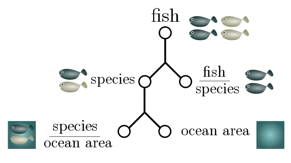
For more complicated Fermi estimates, a good strategy is to break the number into subestimates which are then multiplied together. For instance, if I want to estimate the number of fish in the sea, I might factorise it into the total number of fish species and the number of fish per species:
\[\text{total fish} \sim \text{species} \times \text{fish per species}.\]This sort of factorisation is crying out to be expressed in terms of “generalised units”:
\[\frac{\text{fish}}{\text{world}} \sim \frac{\text{species}}{\text{world}}\times \frac{\text{fish}}{\text{species}}.\]This not only lets us check that our estimate makes sense (units cancel on the RHS to give the LHS) but can suggest further factorisation. The total number of fish species is hard to estimate, but maybe we have a better feeling for how many species there are in a given area of ocean:
\[\frac{\text{species}}{\text{world}} \sim \frac{\text{species}}{\text{area of ocean}}\times \frac{\text{area of ocean}}{\text{world}}.\]The total surface area of ocean is $350$ million km$^2$. It seems reasonable to guess that there is a different species for every $10$ km$^2$ or so, and that a species of fish has on average $10^5$ members. This gives an estimate of
\[\begin{align*} \frac{\text{fish}}{\text{world}} & \sim \frac{\text{species}}{\text{area of ocean}}\times \frac{\text{area of ocean}}{\text{world}}\times \frac{\text{fish}}{\text{species}} \\ & \sim \frac{1}{10 \text{ km}^2} \times (350 \times 10^6 \text{ km}^2) \times 10^5 \\ & = 3.5 \times 10^{12}. \end{align*}\]Somewhat unexpectedly, this is exactly the number quoted in a non-peer-reviewed article. Huh!
Full disclosure. In case you’re suspicious, here is where the intermediate numbers come from. First, you can calculate the total ocean surface from the radius of the earth $r_\oplus = 6300$ km, the surface area of a sphere $4\pi r^2$, and the factoid that $70\%$ of the earth is covered by water. I have no idea if my remaining guesses are accurate. I obtained the number of fish per species by lazily taking the mean of an obscenely successful species (humans, population $\sim 10^{10}$) and a species on the brink of extinction ($\sim 1$). Similarly, for the density, I just took the average of $1$ species per $1 \text{ km}^2$ (seems too large) and $100 \text{ km}^2$ (seems too small). I don’t really trust my intuitions about areal biodiversity, but as often happens with Fermi estimates, you land on your feet!
Exercise 7 (churches). Guess the number of churches in the US.
Hint. A particularly useful intermediate factor is people, both in this problem and in general. The US has a population of around $300$ million.
3.3. KISS
KISS is the old military adage to “Keep It Simple, Stupid”, and it is especially true for Fermi estimates. If you want fast, robust estimates, forget about finesse; just focus on a single important mechanism. You should make simplifying assumptions, ignore subtleties, and strip away distractions to get at that mechanism. In other words, embrace the spherical cow! (Perhaps KISS should stand for “Keep It Spherical, Stupid”.) As I’ll touch on shortly, this also applied to subestimates, and we shouldn’t factorise unless it reduces total uncertainty.
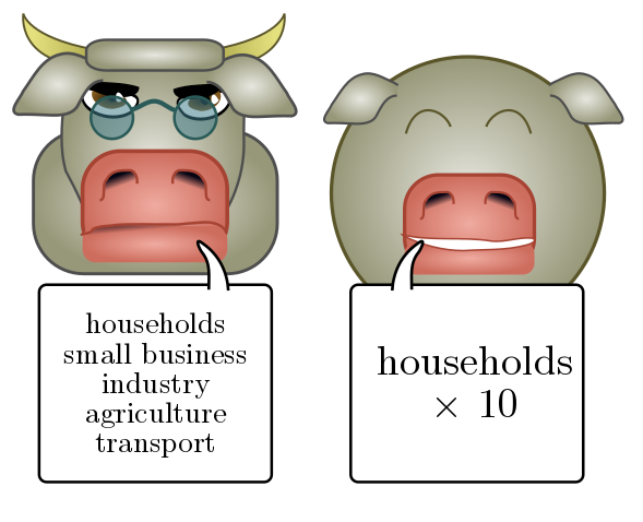
Let’s see how this works in practice. Suppose we want to estimate the annual electricity usage in the greater Vancouver area. (This is an actual question from my PhD comprehensive exam.) We could consider all sorts of separate contributions, e.g. households, small businesses, heavy industry, agriculture, transport, and so on, all of which would involve different estimation strategies. Instead, let’s focus on a single, simple estimate: household power usage. This will make up some fixed fraction of the whole, perhaps $10\%$ or so, so we just multiply by $10$ at the end of the day.
We start with subestimates, factorising our guess using people (rather than households) as an intermediate unit:
\[\frac{\text{power}}{\text{Vancouver}} \sim \frac{\text{power}}{\text{person}}\times \frac{\text{person}}{\text{Vancouver}}.\]The factor “person/Vancouver” is just the population of greater Vancouver, which I happen to know is around $2.5$ million. To estimate individual power usage, we can compare to something familiar like a good ol’ $60$ W globe. I would guess that with light, heat, household appliances, and electronic devices, an individual would use the equivalent of $10$ light bulbs on average, or around $600$ W. Thus,
\[\frac{\text{power}}{\text{Vancouver}} \sim 600 \text{ W} \times (2.5 \times 10^6) = 1.5 \text{ GW}.\]To find the total electricity usage, we multiply by the length of a year, and add an additional factor of $10$ to account for non-household use. In gigawatt hours (GWh), this gives a total energy of
\[\begin{align*} \text{yearly energy use} & \sim 10 \times (365 \times 24 \text{ h}) \times (1.5 \text{ GW}) \approx 1.3 \times 10^5 \text{ GWh}. \end{align*}\]How did we do? Our guess translates to around $500$ PJ (petajoules) per year, and according to this report, British Columbia uses $850–1000$ PJ. Since greater Vancouver has about half the population of the province, we should be spot on!
Exercise 8 (loonie bin). Guess the Canadian government’s federal budget for 2019.
⁂
Exercise 9 (rain power). The annual rainfall in the greater Vancouver region is about $1000$ mm, meaning that all the rain that falls in a year would make a layer $1$ metre deep. Approximately how much energy arrives in the form of raindrops each year?
Hint. You may find Exercise 2 useful. You will need to Fermi estimate the area of greater Vancouver (though you can check with Google).
3.4. Usage notes
Why it works. Fermi approximation is a subtle art. In general, it works because over- and underestimates balance each other out. This is an example of the wisdom of the crowd, where averaging over different types of ignorance yields wisdom, though in this case, the crowd is made up of subestimates! But there is more to it than that. The variance (random variability) of subestimates adds up, and a good rule of thumb is to only factorise into subestimates when the combined uncertainty of these estimates is much smaller than the original. (To be pedantic, by “uncertainty”, we mean “squared error on the logarithmic ruler”.) This is another instance of the KISS principle.
Sanity checks.
You can increase the reliability of a subestimate by performing a sanity check.
Compare to things you know, or manipulate your guess until you can
make that comparison.
For instance, if we guess the Canadian budget is CAD$30
billion, and also know the population (30 million or so), we see this
corresponds to $1000 per person.
Since the government typically spends thousands of dollars per student
on public education (let alone roads, healthcare, defense, etc) this
number is clearly too low.
Web of facts. Aliens cannot sanity check because they don’t know enough about our world. In general, to be a good estimator, you need a web of facts, figures, and intuitions to triangulate your position in estimate space and reduce variance. Books on Fermi problems, e.g. Guesstimation by Weinstein and Adam, usually have a list of handy numbers in the appendix for just this reason. It may feel like cheating, but if you are doing a Fermi problem in real life, also remember that you can make your web of facts much larger using Google!
Nonlinearity. Our final and most subtle failure mode is “nonlinearity”. (Props to lukeprog’s Fermi estimate tutorial for pointing this out.) Our factorisation assumes that subestimates are (a) independent and (b) multiply to give the final answer. Assumption (a) can easily fail. For instance, in our electricity calculation, we assumed that average power usage was independent of population. But average power usage tends to be lower in urban areas because the energy infrastructure is all in one place. Thus, changing one factor (population of a city) will change another (per capita power usage). Sometimes you can take this dependence into account with extra factors, sometimes you can’t.
Assumption (b) fails when the final answer has a different type of functional dependence on its subestimates. A particularly severe example is exponential dependence. Suppose I throw a fistful of quarters onto the ground. What’s the probability they all come up heads? Well, if there are $n$ quarters, and each has a $50\%$ chance of coming up heads, the answer is $(1/2)^n = 2^{-n}$. It seems like all I need to do is count the quarters in a fistful. But here’s the rub: if I’m wrong by three coins, l’ll be off by a factor of $2^3 \approx 10$, which is a whole order of magnitude! If you want a well-defined order of magnitude estimate, back away slowly from exponentials. We’ll explore what you can do with exponential dependence in Exercise 11.
Exercise 10 (people power). Earlier, I guessed (based on a hunch) that individuals use around $600$ W (or $10$ light bulbs) on average. Let’s check this a few different ways.
(a) Ask some friends to guess, and take the geometric mean of their answers.
(b) Next, sanity check my guess or the answer you got in (a).
(c) Finally, ask Google. How did I do? How did your friends do?
⁂
Exercise 11 (jumping mugs). Exponentials may prevent us from doing reliable order of magnitude estimates, but they do not prevent us from drawing physical conclusions. Let’s see how likely your mug is to jump spontaneously into the air.
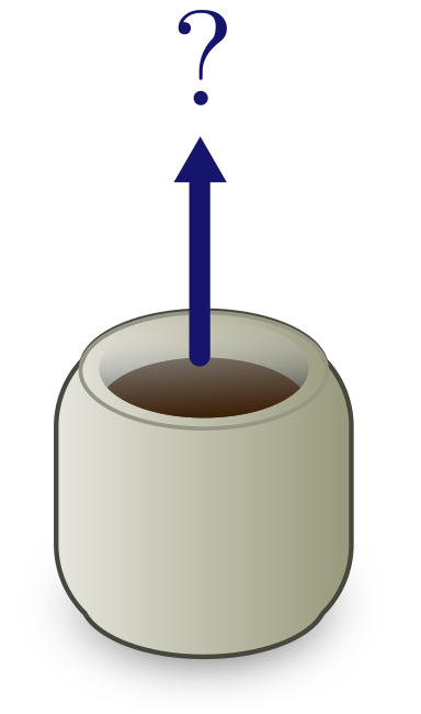
(a) Estimate the number of atoms $n_C$ in a mug of coffee.
Hint. Recall that Avogadro’s number $N_A = 6 \times 10^{23}$ is the number of atoms in $12$ g of carbon-12. We will derive this in Exercise 19!
(b) Very roughly, what is the probability the mug jumps spontaneously into the air?
Hint. Atoms move in random directions. The coffee will spontaneously jump if all the atoms in the cup are moving up.
(c) A mug cycles through about $10^{14}$ random configurations per second. If you watch your mug until the entropic heat death of the universe (about $10^{100}$ years away) are you likely to see it jump?
(d) Given that $n_C$ can vary by an order of magnitude, how does the probability of spontaneous jumping vary? Does it change your conclusion in (c)?
In a sense, the Second Law of Thermodynamics is just a generalisation of this exercise. But we’ll save that for another day!
4. Random walks
Although they are ripe for hacking, both dimensional analysis and Fermi approximation are fairly conventional back-of-the-napkin methods. In contrast, our final hack — random walks — is almost never seen outside of probability or statistical physics courses. While our treatment is elementary, it is still a step up from the first two tutorials, and is perhaps best left to a second reading. But, as always with a good hack, our reward is applications: we will find the length of the E. coli genome; see why unmanned spacecraft aren’t programmed to avoid asteroids; explain whether you should walk or run in the rain; and finally, prove the existence of atoms and weigh them. It’s action-packed!
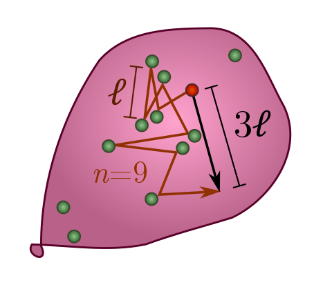
Random walks: an elementary approach. Imagine an atom jiggling around randomly in a hot gas. On average, it travels some distance $\ell$ between collisions. How far does it travel after $n$ collisions? Given some fairly mild assumptions, the answer is surprisingly
\[d \sim \ell \sqrt{n}.\]If it travelled in a straight line, the distance would be $d = \ell n$. Randomness apparently reduces the linear power $n^1$ to a square root $n^{1/2}$.
To see how this happens, let’s start watching an atom as it bounces around, and label its displacement after the $i$th step $\vec{s}_i$. The arrow on top reminds us that displacement is a vector, with an associated direction in space, and not just a number. Since the distance between collisions is on average $\ell$, we have $|\vec{s}_i| = \ell$ and hence $|\vec{s}_i|^2 = \ell^2$. After $n$ collisions, the total displacement is
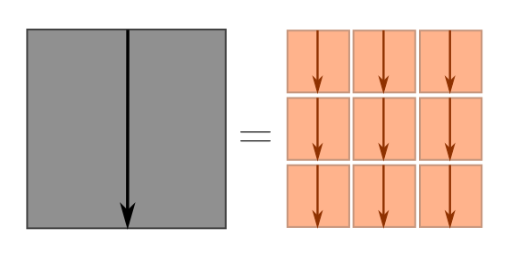
\[\vec{x} = \vec{s}_1 + \vec{s}_2 + \cdots + \vec{s}_n.\]How can we calculate the length of $\vec{x}$? The trick is to square it, yielding
\[|\vec{x}|^2 = (\vec{s}_1 + \vec{s}_2 + \cdots + \vec{s}_n)^2 = |\vec{s}_1|^2 + |\vec{s}_2|^2 + \cdots +|\vec{s}_n|^2 + \text{cross-terms}.\]This is a generalisation of the familiar algebraic fact that
\[(x+y)^2 = x^2 + y^2 + 2xy = x^2 + y^2 + \text{cross-terms}.\]We can picture what’s going on using squares.
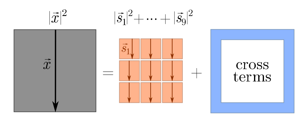
The cross-terms are things like $\vec{s}_1 \cdot \vec{s}_2$, $\vec{s}_2 \cdot \vec{s}_3$, and so on. Although it obey similar algebraic properties to normal multiplication, the $\cdot$ in terms like $\vec{s}_1\cdot \vec{s}_2$ has a special geometric interpretation: it tells us how aligned the vectors $\vec{s}_1$ and $\vec{s}_2$ are. Since these are random steps, we don’t really care about any two specific steps, but rather how aligned they are on average. If vectors are not aligned on average, then the cross-terms vanish, and as claimed we will have
\[d^2 \sim s_1^2 + s_2^2 + \cdots s_n^2 = n\ell^2 \quad \Longrightarrow \quad d \sim \ell \sqrt{n},\]where the $\sim$ means “roughly speaking”. For dimensional analysis, “roughly speaking” meant “up to numbers”, and for Fermi estimates, “up to a factor of $3$”. Here, “roughly speaking” means “on average”. In our earlier picture, the blue terms vanish, and we just have the big square equal to the sum of little squares.
So, under what circumstances will consecutive steps tend not to align? Two conditions will be enough:
- Steps are unbiased, i.e. don’t prefer any particular direction. If they are biased, say the walker likes to head south, then there is a preferred direction and the steps tend to align with it.
- Steps are uncorrelated, i.e. consecutive steps don’t know about each other. If the walker likes to follow one step with another in the same direction, then steps will tend line up, even if there is no preferred direction.
You can play with these conditions for a simple example in Exercise 12. In all our random walks below, however, the walk is unbiased and uncorrelated to good approximation, and hence steps are unaligned.
Speed and diffusion. If a random walker moves with speed $v$, an average step takes time $\tau = \ell/v$. After a total time $t$ has elapsed, the random walker will take around $t/\tau$ steps, and will therefore wander a distance
\[d \sim \ell \sqrt{n} = \ell \sqrt{\frac{t}{\tau}} = \sqrt{\ell v}\cdot \sqrt{t} = \sqrt{Dt}.\]We will call $D = \ell v$ the diffusion coefficient. It’s important to note that “average distance” is a bit of a misnomer. We really mean the average spread of distance travelled. In time $t$, an individual walker will explore a region of size $\propto \sqrt{t}$, while a batch of walkers released from the same point will fan out to cover that region.
Exercise 12 (heads and tails). Take a fair coin and start flipping it. The outcome of the $i$th flip is $s_i = \pm 1$, with $+1$ for tails and $-1$ for heads, and the sum of $n$ flips is $x$. To square $x$, we really do just multiply and expand, with
\[x^2 = (s_1 + \cdots + s_n)^2 = s_1^2 + \cdots s_n^2 + 2 \left[s_1 s_2 + \cdots + s_{n-1}s_n\right].\]We can think of $x$ as describing the position of a random walk on the number line.
(a) For a fair coin, show that on average, $s^2 = 1$.
(b) Consider two fair coin flips, $s$ and $s’$. Show that $ss’ = +1$ with probability $1/2$ and $ss’ = -1$ with probability $1/2$. Conclude that, on average, $ss’$ vanishes. (More carefully: if I add up the results of many experiments and divide by the number of experiments, the answer will tend towards $0$.)
(c) Combining the last two arguments, argue that after $n$ coin flips, the random walk tends to spread a distance $\sqrt{n}$ around the origin, with $x \sim \sqrt{n}$.
Let’s now briefly consider two ways for the random walk description to fail: bias and correlation. A coin has bias when there is a probability $p \neq 1/2$ of getting $+1$ (tails), and $q = 1- p$ of getting $-1$ (heads). Two flips $s$ and $s’$ are correlated with $c$ if on average
\[ss' \sim c + (p-q)^2.\]First, we explore bias.
(d) Explain why $s^2 = 1$ even if the coin is biased or flips are correlated.
(e) For biased but uncorrelated coin flips, derive
\[d^2 \sim n + n(n-1)(p-q)^2.\]Let’s end with a very simple example of correlation. Consider an unbiased coin with correlation $c$ between successive flips only.
(f) Check that the walk still obeys $d \propto \sqrt{n}$.
4.1. Polymers
Random walks not only apply to processes in time, but also in space. The most important example is polymers: long, jointed chains of molecules which can often be described by a random walk. In this case, the step length $\ell$ is the persistence length of the polymer, the distance the polymer remains approximately straight. After a persistence length, the chain will forget which way it is pointing and choose a new, uncorrelated direction. We’ll look at a biological application to the biggest, baddest, most biologically indispensable polymer of them all: DNA.
Every cell in an organism contains a copy of its building instructions in DNA form. Most organisms are eukaryotes, meaning each cell has a special chamber called the nucleus for storing DNA, but in prokaryotes (such as bacteria), the DNA just freely floats in the cellular soup. Either way, if the container ruptures, the tightly coiled DNA will spill out and form a random walk of approximately straight chunks. The persistence length is $\ell = 48$ nm, which corresponds to about 140 base pairs (bp). (A base pair is just one of the dumbbell components of the double helix.)
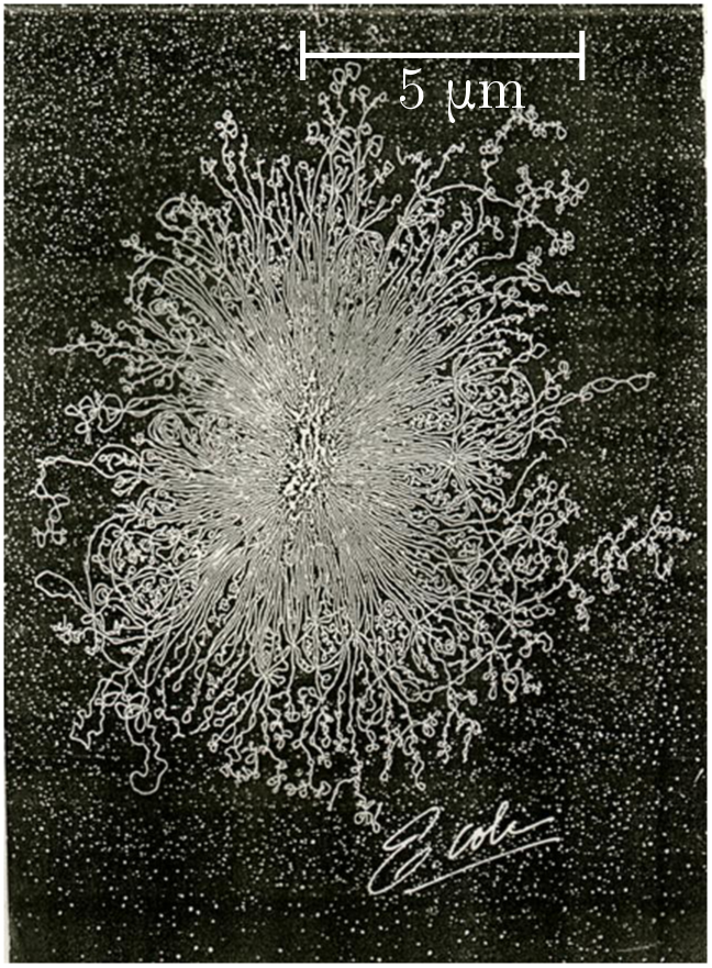
In the photo above, the nucleus of a single-celled Escherichia coli (E. coli) bacterium has ruptured. From the spill, we can estimate the length of its genome! The DNA covers a region with radius
\[d \approx 5 \,\mu\text{m} = 5000 \text{ nm}.\]Then, using the chunk length $\ell = 48$ nm, we guess that the number of chunks is
\[n \sim \frac{d^2}{\ell^2} \approx \left(\frac{5000}{48}\right)^2 \approx 1.1 \times 10^5.\]Multiplying by the number of base pairs per chunk, we estimate a genome length
\[L_\text{gen} \sim n \times (140 \text{ bp}) \approx 1.5 \times 10^6 \text{ bp},\]or $1.5$ Mbp. A careful count gives $4.6$ Mbp, so we are just within an order of magnitude!
Exercise 13 (gone fishing). Wandering the shipyards one day, you notice a rusty old anchor and chain, probably from a decommissioned fishing vessel. The chain is piled haphazardly on the dock. The links are around $7$ inches in length, and the pile is $4.7$ m across. What is the approximate length of the chain?
4.2. Bumping into things
Collisions occur when objects happen to be in the same place at the same time. If you want to keep track of what is entering your space, imagine that you sweep out an envelope as you move. The bigger you are, the more likely you are to collide with things. But you are more likely to collide with elephants than fleas! You also want to take into account the size of the objects you might be running into.
The formal way of doing this is a scattering cross-section $\sigma$. The basic idea is that if you sweep out a “collision cylinder” with cross-section $\sigma$, and the centre of another object lies in the cylinder, a collision will occur. The cross-section $\sigma$ takes into account both your size and the size of the objects you collide with. If you move a distance $\lambda$, and have scattering cross-section $\sigma$ with respect to elephants (or whatever it is you are worried about colliding with), your collision cylinder will have volume
\[V = \lambda\sigma.\]If we know the number of colliding objects (e.g. elephants) per unit volume in the vicinity, we can estimate the number of collisions. For instance, if there are $n$ elephants per unit volume, then on average, you will collide with $nV = n\sigma \lambda$ elephants as you move a distance $\lambda$.
Let’s do some very simple examples of cross-sections. Picture yourself as a sphere of radius $R$, worried about colliding with spheres of radius $r$. You can show in Exercise 14 that the scattering cross-section is
\[\sigma = \pi (R+r)^2.\]This means in particular that if you are much larger than the spheres you are bumping into, the cross-section is approximately $\pi R^2$, and if you are much smaller, it is approximtely $\pi r^2$. If you are colliding with spheres of the same size, then the scattering cross-section is
\[\sigma = \pi (2R)^2.\]This covers most of the cases we will be interested in!
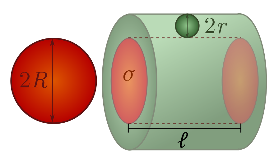
Mean free path. Now, back to our regular programming: random walks in gases. We would like to determine the step length $\ell$ for the random walk executed by colliding particles, assuming they are all spheres of radius $r$. The method is simple. We just draw a collision cylinder until the number of expected collisions is $1$, then call it a day:
\[1 = n V = n \ell \sigma \quad \Longrightarrow \quad \ell = \frac{1}{n\sigma} = \frac{1}{\pi n (2r)^2}.\]Hopefully this makes sense. We want $\ell$ to be average distance between collisions, and this is exactly what the collision cylinder calculates when we set the number of collisions equal to one. The fancy name for distance between collisions is mean free path, but we will use this sparingly.
As a simple example, we can estimate the average distance between collisions of air molecules at room temperature ($300$ K) and atmospheric pressure ($100$ kPa). The trick is to exchange temperature and pressure for number per unit volume using the ideal gas law (Exercise 3):
\[PV = \mathcal{N}k_B \mathcal{T} \quad \Longrightarrow \quad n = \frac{\mathcal{N}}{V}= \frac{P}{k_B \mathcal{T}},\]where $n = \mathcal{N}/V$ is the number of air particles per unit volume. To find $\lambda$, we also need the size of an air molecule. Most of it is nitrogen, and a little oxygen, with average diameter $2r = 4 \times 10^{-10}$ m. We can plug all our numbers in, along with Boltzmann’s constant, to find the mean free path:
\[\ell = \frac{1}{\pi n (2r)^2} = \frac{k_B\mathcal{T}}{\pi P (2r)^2} = \frac{(1.38 \times 10^{-23})300}{\pi (100\times 10^3)(4 \times 10^{-10})^2} \text{ m} \sim 80 \text{ nm}.\]So, on average an air molecule travels around $80$ nm between collisions, a couple of hundred times its own diameter. In Exercise 15, you’ll see how fast air molecules diffuse.
One final technical point. Most of this collision cylinder technology assumes that we are colliding with stationary objects. If they are stationary on average, that is, there is no preferred direction, then the same estimates still work provided you are small enough, and the colliders are low enough density, that staying still will lead to very few collisions. But when you are too big or they are too dense, remain still and you will collide with many objects! This is pressure. To understand how very large objects interact with a dense bath of tiny, randomly moving ones, it’s better to use thermodynamics than cylinders.
Exercise 14 (smashing spheres). Consider two spheres of radius $R$ and $r$.
(a) Show that if the centres come within a distance $R+r$, they will collide.
(b) Explain why the scattering cross-section is $\sigma = \pi (R+r)^2$.
(c) Conclude that, if $R \gg r$, then $\sigma \approx \pi R^2$.
⁂
Exercise 15 (asteroid belt). The asteroid belt is a donut-shaped blob of asteroids (small rocky bodies) between Jupiter and Mars. The blob extends from $2.2$ to $3.2$ astronomical units (AU) away from the sun, where
\[1 \text{ AU} =15 \times 10^8 \text{ km}\]is the sun-to-earth distance. There are about $25$ million large asteroids, with average diameter around $10$ km. Although this sounds like a dangerous place, Wikipedia states that “numerous unmanned spacecraft have traversed it without incident”. Let’s see why!
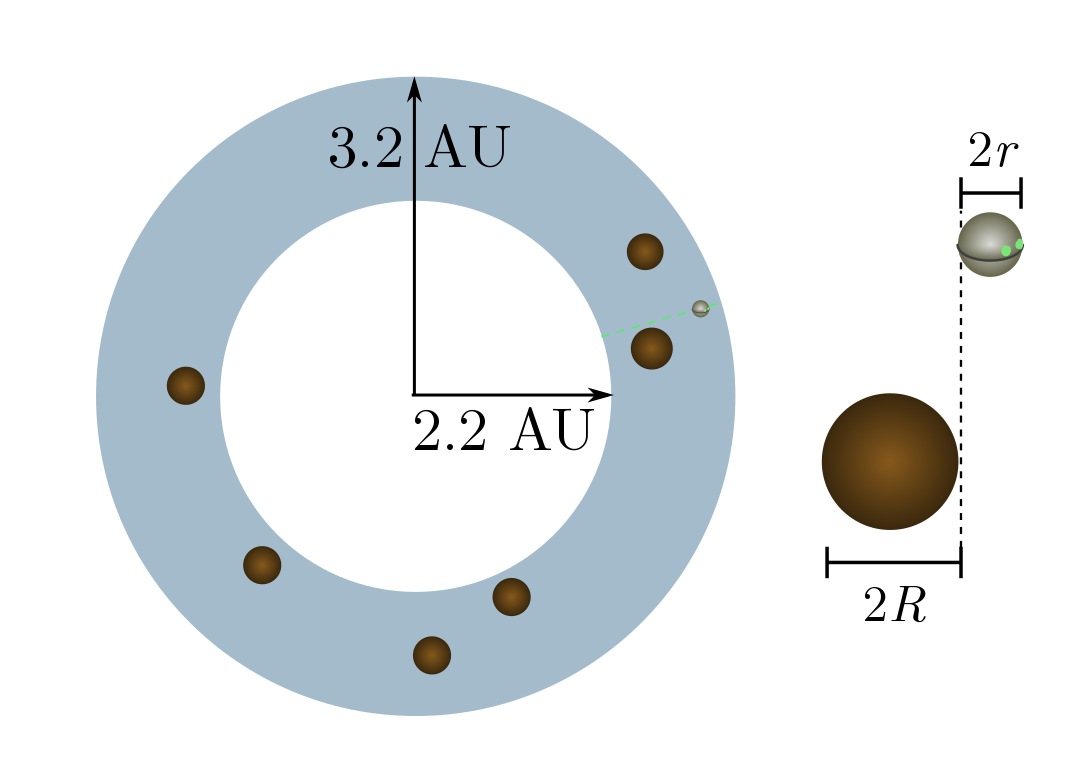
(a) For simplicity, let’s flatten the donut into a ring with inner radius $2.2$ AU and outer radius $3.2$ AU. What the density $n$ of asteroids per unit area?
(b) Cross-sections are now going to be lengths rather than areas, since we are living in two dimensions. Explain why a circle of radius $r$ colliding with circles of radius $R$ will have cross-section $R + r$.
(c) A $20$ km-wide asteroid is much, much larger than an unmanned spacecraft. Calculate the mean free path, and explain why the spacecraft will almost never collide with an asteroid.
⁂
Exercise 16 (equipartition and air time). People often say that “temperature is just atomic motion”. This is shorthand for “temperature is just average kinetic energy per particle”, which we write as
\[\epsilon_\text{avg} \sim k_B \mathcal{T},\]where $\epsilon_\text{avg}$ is the kinetic energy per particle and $k_B$ is Boltzmann’s constant. This is a simple version of a deep result called the equipartition theorem, and for my money, it is the clearest way to interpret temperature microscopically.
(a) Show that if the particles have mass $m$, the average speed is
\[v_\text{avg} \sim \sqrt{\frac{k_B \mathcal{T}}{m}}.\](b) Using the collision cylinder method, compute the diffusion constant $D = \ell v$ in a gas with pressure $P$ and temperature $\mathcal{T}$, consisting of particles of mass $m$ and size $r$. You should find that
\[D \sim \frac{(k_B \mathcal{T})^{3/2}}{\pi \sqrt{m} P (2r)^2 }.\](c) The average mass of an air molecule is $m = 5 \times 10^{-26}$ kg. (Once again, this is slightly larger than the mass of an N$_2$ molecule, since air is mostly nitrogen plus some heavier elements.) Estimate how long it will take an air molecule near your head to reach the wall.
4.3. Rainy day dilemma
We can apply our collision cylinder technology to solve an age-old problem: should you walk or run in the rain? (In a city like Vancouver, this is a question of practical import.) We will present a simple and original argument which models people as spheres; see Exercise 16 for the conventional approach which models people as boxes. So, you are a sphere of radius $R$ stuck in a rainstorm, with shelter a distance $d$ away, which you move towards at some speed $u$. The rain consists of tiny balls of water falling directly down (no wind) at speed $v$, with some number of drops $n$ per unit volume. The speed and density can change with height, but we’re only interested in these quantities near the ground, so we are at liberty to imagine that they are constant everywhere.
It seems like we might have to modify collision cylinders to take the velocity of the rain into account, but there’s a beautiful shortcut: we just think about everything in the reference frame of the rain. From the rain’s perspective, you travel vertically up at speed $v$, and with a horizontal velocity component $u$ towards the shelter (represented as a vertical line a distance $d$ away). The question is: does the number of drops you collide with on your way to shelter depend on $u$? If it doesn’t, you may as well walk.
The answer is obviously yes, since if you stand still, you will get infinitely soaked, but let’s explore this with a little more care. If you move at speed $u > 0$, you arrive at shelter in time $t = d/u$. Hence, your path has length
\[\lambda = \sqrt{(vt)^2 + (ut)^2} = d\sqrt{1 + (v/u)^2}.\]Since the drops are small, your cross-section is $\sigma = \pi R^2$, and the number of drops you collide with is then
\[nV = n \sigma \lambda = \pi nR^2d\sqrt{1 + (v/u)^2}.\]To make this as small as possible, you should make $u$ as large as possible. In other words, run for shelter!
This is particularly clear when the rain falls much faster than you run, with $v/u \gg 1$. In this case, $\sqrt{1 + (v/u)^2} \approx \sqrt{(v/u)^2} = v/u$, and hence
\[n V \approx \pi n R^2d \cdot \frac{v}{u} = (\pi n R^2 v)t.\]How wet you get is directly proportional to how much time you spend in the rain.
Exercise 17 (the soggy box). Let’s now make a slightly more realistic model of a person: a box of height $h$, width $w$, and breadth $b$. For simplicity, suppose there is no wind, so the rain falls directly down, and shelter is a distance $d$ away. The collision cylinder will now be made up of two pieces, associated with the front and top of the box.
(a) Argue that the volume of the collision cylinder for the front of the box does not depend on running speed $u$. Is this consistent with our original observation that a stationary sphere will get infinitely wet?
Hint. You may find trigonometry useful.
(b) Show that the collision cylinder for the top of the box has a volume proportional to $t$.
(c) Find the conditions for $h, w$ and $d$ under which you should run for cover. When are they likely to be satisfied for a human?
We reach similar conclusions to the sphere, though I personally find the sphere argument quicker and cleaner.
⁂
Exercise 18 (wet and windy). When the wind blows, it imparts a horizontal velocity to the rain. As above, we consider a sphere seeking shelter a distance $d$ away.
(a) If the wind blows away from shelter, explain why you should run as fast as possible.
(b) Suppose the wind is blowing towards shelter with a horizontal velocity $u’$, and has downward velocity $v$. Demonstrate that there is a finite optimal speed to move towards shelter, $v^2/u’$. If it’s very windy, it may be better to walk!
4.4. Brownian motion
Before the 20th century, the notion that matter was made of tiny, indivisible lumps was regarded with skepticism. But in 1905, long before we could see atoms with microscopes, a Swiss patent clerk came up with a brilliant indirect method for proving their existence. The clerk was none other than Albert Einstein, and his proof uses random walks. Let’s see how he did it!
We start by pouring a viscous fluid into a tall container of volume $V$. The fluid is made up of $\mathcal{N}$ particles at temperature $\mathcal{T}$, and we assume it is dilute enough to be described by the ideal gas law (Exercise 3). Now plonk some large, easily visible particles into this fluid, for instance pollen grains, of radius $r$ and mass $m$. The pollen grains will randomly collide with particles in the fluid, executing a random walk as they do so. If the grain is much larger than the fluid particles, we can treat the latter as points, so the collision cylinder has cross-section $\sigma = \pi r^2$.
Counting the number of particles is hard, but measuring the temperature is easy. Like the air example above, we can use the ideal gas law to swap volume and number for pressure and temperature:
\[PV = \mathcal{N} k_B\mathcal{T} \quad \Longrightarrow \quad \ell = \frac{V}{\mathcal{N}\sigma} = \frac{k_B\mathcal{T}}{P \pi r^2}.\]Since the container is tall, the pressure profile $P$ changes with height. But if we leave the pollen grains alone for long enough, they will fall down and settle into equilibrium roughly where pressure from the fluid balances weight, with
\[P = \frac{F}{A} \sim \frac{mg}{\pi r^2},\]and hence
\[\ell \sim \frac{k_B\mathcal{T}}{mg}.\]Recall that the diffusion coefficient $D = \ell v$ is directly related to the meandering of the pollen grain over time, with $d^2 \sim Dt$. To calculate this coefficient, we still need to work out the velocity, $v$, but here is the clever part: since our fluid was viscous, and assuming the grains move slowly, we can apply Stokes’ law! Since the grains are in equilibrium, it’s reasonable to guess that their velocity is the terminal velocity
\[v_{\text{term}} = \frac{mg}{6\pi \mu r},\]where $\mu$ is the viscosity. Putting it all together, we predict a diffusion coefficient
\[D \sim \ell v_{\text{term}} = \frac{k_B\mathcal{T}}{6\pi \mu r}.\]This short argument ignores the fact that grains can jitter up and down, as explained in the appendix. But our method gives the right answer, and in the spirit of cheeky hacker approximation I will let it stand.
The expression for $D$ is called the Stokes-Einstein relation, and it is one of the major results of Einstein’s PhD thesis. The weight of the pollen cancels out, leaving a diffusion constant which grows with temperature but is inversely proportional to particle size. Big particles jiggle less, hot fluids jiggle more, and things look the same on Mars!
The jiggling of grains in a fluid was first observed by Robert Brown, hence the name Brownian motion. (It should perhaps be called Lucretian motion, since Lucretius observed the zigzag motion of dust particles and attributed it to atoms — in 60 BC!) Although Brownian motion is best explained by atoms, Einstein’s genius was to extract specific and testable predictions, which Jean Perrin confirmed experimentally in 1908. Both Perrin and Einstein received Nobel prizes, in part for this work. We’ll end with one of the practical applications Einstein suggested and Perrin carried out: calculating Avogadro’s constant.
Exercise 19 (Avogadro’s constant). You may have seen the ideal gas law (Exercise 3) in its chemistry guise:
\[PV = n_\text{mol} \mathcal{R} \mathcal{T},\]where $n_\text{mol}$ is the number of particles measured in mol, and $\mathcal{R}$ is the ideal gas constant,
\[\mathcal{R} = 8.3 \, \text{ J / K mol}.\]Recall that one mole is $N_A$ particles, where $N_A$ is Avogadro’s constant, the number of carbon atoms in a $12$ g lump. But Avogadro didn’t know his own constant! His big contribution was a related observation called Avogadro’s law:
Equal volumes of gas, at equal temperature and pressure, contain the same number of molecules.
This was a prescient insight into the atomic nature of matter, anticipating the ideal gas law by 45 years. It underpins the utility of the mole, which is why Perrin named the constant he first measured in Avogadro’s honour.
Determining the number of molecules in a sample of gas is the same as weighing a molecule. This turns out to be hard! But it is easy to measure the volume of the gas (place it in a container of fixed volume), the pressure (use a barometer), the temperature (a thermometer), and the number of mol (chemistry). That makes it fairly easy to measure the ideal gas constant $\mathcal{R}$, and indeed, it was calculated as early as 1850 due to the combined efforts of Henri Regnault and Rudolf Clausius. So we will take $\mathcal{R}$ as a given, and leave ourselves the much harder task of weighing atoms.
(a) By equating the different forms of the ideal gas law, show that $N_A = \mathcal{R}/k_B$.
To weigh atoms and molecules, all we need to do is divide the molar mass by $N_A$. Perrin and Einstein gave the first modern estimates of Avogadro’s number using Brownian motion, and we will follow in their footsteps. (Remarkably, Einstein, the master hacker, proposed no fewer than five methods for determining $N_A$.)
(b) Suppose a spherical particle jiggles a distance $d$ in time $t$ due to Brownian motion. Using the Einstein-Stokes relation, show that
\[N_A \sim \frac{t}{d^2}\cdot \frac{\mathcal{R}\mathcal{T}}{6\pi \eta r}.\]Up to factors, this is the last equation in Einstein’s famous paper on Brownian motion!
Perrin used Einstein’s method to determine $N_A$. He painstakingly prepared tiny spheres of a resin called gamboge, then dropped them into warm water and watched them dance. The tracks of a resin particle ($r = 0.52 \times 10^{-6}$ m) from Perrin’s data set is shown below. The dots are observations made every $30$ s, and divisions on the graph are ruled at intervals of $3.125 \times 10^{-6}$ m.
(c) Use the tracks to estimate Avogadro’s constant. The temperature of the water was around $\mathcal{T} = 290$ K, with viscosity $\eta \approx 0.0011$ kg/m s.
As you probably know from chemistry class, the official value is $N_A = 6.02 \times 10^{23}$. Hopefully you got something close in the last question! We can finally use this to weigh a molecule. As a bonus, we can weigh protons and neutrons as well.
(d) Estimate the mass of a carbon atom.
(e) Naturally occuring carbon is mostly carbon-12, which has $12$ nucleons (protons and neutrons of approximately equal mass) in the nucleus. How heavy is a nucleon?
I think this is pretty neat. From watching resin balls jiggle in water, we can work out the mass of a proton!
5. Conclusion
I hope I’ve convinced you that the hack is strong with napkins. Every single thing we did — from pendulum periods to the ideal gas law, power usage to proton mass — required, at most, a little pre-calculus math and solid command of a napkin hack. There is obviously great power in simple techniques, and we have only scratched the surface! Physics is brimming with napkin algorithms, just waiting for hackers to explore, exploit and explain, to guide us towards that apotheosis of hacker spirit Stallman describes:
Look how wonderful this is. I bet you didn’t believe this could be done.
So, why aren’t we blowing more gourds with high-leverage, low-tech hacks? Probably, mostly, the inertia of convention. For instance, we’re taught to analyse mechanics problems by adding up vectors, and electricity problems by drawing circuits. These methods are well-adapted, but this is precisely what makes them low leverage! It might surprise you to learn that we can add vectors to describe the flow of electricity and draw circuits to solve mechanics problems. We are bound by convention and familiarity to the typical use case, but there’s often something remarkable just around the corner.
Other myths are at play here. One of the most dangerous is that the only real tool is calculus and its tributaries, and before students master these dark arts, they must settle for useless caricatures of natural law. This assertion is nonsense, as the examples above conclusively demonstrate. Similarly, application and experiment are often deemed too difficult for quantitative treatment, though they are the lifeblood of the physical sciences. Once again, this is just plain false!
In summary, we are dealing with the age-old problem of tradition, the fact that conventions tend to be received and transmitted without question. There is a great deal that is good in the received wisdom, but also a great deal of limitation and falsehood. In the words of Cyprian of Carthage,
Custom without truth is the antiquity of error.
Hacker spirit — with its willingness to peek around corners and its healthy disrespect for authority — is the perfect antidote for custom without truth.
References
- Physical Biology of the Cell (2013), Phillips, Kondev, Theriot, Garcia. A superb textbook on the physical and mathematical aspects of cells, imbued with hacker spirit. This is the source for our E. coli estimate.
- “Fermi estimates” (2013), lukeprog. A short and high-powered introduction to Fermi estimates.
- Street-Fighting Mathematics (2010), Sanjoy Mahajan. An excellent text covering dimensional analysis and Fermi estimates at an undergraduate level.
- “Investigations on the theory of Brownian movement” (1905), Albert Einstein. Einstein’s brief but revolutionary paper on Brownian motion.
- Guesstimation (2008), Weinstein and Adam. A giant compendium of Fermi questions and corresponding solution strategies. Silly but fun.